
“PostgreSQL is not a database with extensions.
It is an extensible data platform that happens to speak SQL.”
Most PostgreSQL tutorials end where the interesting work begins.
Once you know how to SELECT, JOIN, and
GROUP BY, you have mastered perhaps twenty percent of what
PostgreSQL can do. The remaining eighty percent — geospatial queries,
semantic search, real-time notifications, fuzzy matching, vector
embeddings, distributed coordination, and more — lives in a ecosystem of
extensions, index types, and language features that most practitioners
never discover.
This book is a guided tour of that other eighty percent.
Each chapter is built around a concrete engineering problem faced by the fictional city of Portsmith and its data platform team. We store business directories as semi-structured JSON documents. We route emergency services using geospatial proximity queries. We build a job queue with no message broker. We search municipal records with fuzzy matching that survives typos and OCR errors. We expose the entire platform as a REST API with zero application code.
Every chapter follows the same structure: synthetic data is generated first, giving you a realistic dataset to work against, and then a series of exercises walks you from first principles to production-ready technique. The exercises are written to be done — not just read.
By the end, you will see PostgreSQL not as a place to store rows, but as a programmable data infrastructure layer capable of doing work that most teams reach for separate specialized systems to handle.
What you will need:
pg-ripple, one for
pgColumnar, kept apart so neither can affect the other) —
setup for all four environments covered in Appendix ASELECT,
INSERT, JOIN, GROUP BY)Chris Lee
Edition 1.0 — September 12, 2026
“A schema is a prediction about the future. JSONB lets you hedge.”
Relational databases enforce a contract: every row in a table has exactly the same columns. That contract is usually a feature — it catches mistakes and makes queries predictable. But sometimes you genuinely don’t know what columns you’ll need until the data arrives. A business directory is a good example. A restaurant has hours, cuisine, and a reservations policy. A hardware shop has trade accounts and parking. A hotel has star ratings and room types. Forcing them all into the same set of columns means drowning in NULLs or building a rats’ nest of one-to-many extension tables.
PostgreSQL’s JSONB type lets you store arbitrary JSON
documents in a column while keeping the rest of your row fully
relational. It is not a NoSQL escape hatch — it is an indexed,
queryable, patchable document field that sits inside a SQL table. You
can WHERE on it, join against it, aggregate over it, and
update individual keys without rewriting the whole document.
This chapter works through all the operators and patterns you’ll reach for most often. The exercises are short. Run every one, then try a variation of your own.
Portsmith’s city council maintains a public business directory. Every business gets a short relational record — an ID, a name, an address, and a neighbourhood — but the supplementary detail varies so widely by business type that a single fixed schema would be unworkable.
The businesses table therefore stores all of that
variable metadata in a details JSONB column. Each business
category contributes its own keys:
| Category | JSONB keys present |
|---|---|
restaurant |
cuisine, price_range, rating,
hours, tags,
accepts_reservations, outdoor_seating |
retail |
subcategory, rating, hours,
tags, payment_methods,
has_parking |
service |
subcategory, rating, hours,
tags, appointment_required,
specialties |
accommodation |
subcategory, star_rating,
rating, hours, amenities,
room_types, price_per_night |
entertainment |
subcategory, rating, hours,
tags, live_music,
age_restriction |
The hours value is itself a nested object keyed by day
of week (mon–sun). Each day is either
null (closed) or
{"open": "HH:MM", "close": "HH:MM"}. Several businesses
also carry optional keys that appear only for their category, like
social (social media handles), happy_hour, or
approved_brands.
This heterogeneity is intentional — it is what makes the data a good vehicle for learning JSONB operators.
By the end of this chapter you will be able to:
->,
->>, and #>>, and explain why the
operator choice changes the result type.@> and
the key-existence operators ?, ?|, and
?&.jsonb_set and the
|| merge operator without rewriting the whole column.jsonb_array_elements and aggregate the results.jsonb_path_query expressions to filter on nested
values.If PostgreSQL 16 is not already installed:
sudo apt update
sudo apt install -y postgresql-16 postgresql-client-16
Confirm the server is running:
pg_lsclustersYou should see a cluster at version 16 in the online
state.
sudo apt install -y python3.12 python3.12-venvCreate a virtual environment in the book’s working directory and install the PostgreSQL driver:
python3.12 -m venv .venv
source .venv/bin/activate
pip install "psycopg[binary]"
Note:
psycopg(version 3) is the modern Python driver for PostgreSQL. It is not available as anaptpackage for Python 3.12, so we install it via pip into the virtual environment. The[binary]extra bundles a pre-compiled C extension so you don’t needlibpq-dev.
# Create a role matching your OS user (skip if it already exists)
sudo -u postgres createuser --createdb "$(whoami)"

# Create the portsmith database
createdb portsmithFrom the book/ directory, with the virtual environment
active:
python data/ch01_seed.pyExpected output:
Connecting to: dbname=portsmith
Creating schema …
Inserting 48 businesses …
Done — 48 rows in businesses.Open a psql session:
psql portsmithRun these checks. If all three pass, the data is correct.
Check 1 — Row count and column types:
\d businesses Table "public.businesses"
Column | Type | Collation | Nullable | Default
---------------+---------+-----------+----------+------------------------------------
id | integer | | not null | nextval('businesses_id_seq'::regclass)
name | text | | not null |
address | text | | not null |
neighbourhood | text | | not null |
details | jsonb | | not null |Check 2 — Counts by neighbourhood:
SELECT neighbourhood, COUNT(*) AS businesses
FROM   businesses
GROUP  BY neighbourhood
ORDER  BY neighbourhood;
neighbourhood | businesses
--------------------+------------
Harbour District | 9
Industrial Port | 7
Northgate | 9
Old Town | 9
Riverside | 9
University Quarter | 5
(6 rows)Check 3 — Counts by category:
SELECT details->>'category' AS category, COUNT(*) AS businesses
FROM   businesses
GROUP  BY category
ORDER  BY category;
category | businesses
-----------------+------------
accommodation | 5
entertainment | 6
restaurant | 15
retail | 12
service | 10
(5 rows)If all three match, proceed to the exercises.
JSONB has two families of accessor. The arrow operators
(-> and ->>) navigate one key at a
time. The path operator (#>>) jumps straight to a
deeply nested value. The difference between them is the type
they return.
1.1 — Arrow operators
Run these two queries and compare the result types:
-- -> returns JSONB
SELECT name,
       details -> 'rating' AS rating_jsonb
FROM   businesses
LIMIT  5;
-- ->> returns TEXT
SELECT name,
details ->> 'rating' AS rating_text
FROM businesses
LIMIT 5;Look carefully at the column headings in psql — one will
show jsonb, the other text. This distinction
matters the moment you try to do arithmetic:
-- This works: cast text to numeric
SELECT name,
       (details ->> 'rating')::numeric AS rating
FROM   businesses
ORDER  BY rating DESC
LIMIT  5;
name | rating
-------------------------+--------
Lighthouse Bookshop | 4.9
Finch & Sons Barbers | 4.9
Portsmith Vet. Clinic | 4.8
River Bend Bakery | 4.8
Quarter Note Jazz Club | 4.8
(5 rows)Key point: Use
->when you want to keep working with JSONB (e.g., to navigate deeper). Use->>when you need the final value as text for comparisons, casting, or display.
1.2 — The path operator #>>
Navigating nested keys with chained -> quickly
becomes unreadable. The path operator takes an array of keys and returns
the leaf as text in one step.
-- Chained arrows (verbose)
SELECT name,
       details -> 'hours' -> 'fri' ->> 'close' AS friday_close
FROM   businesses
WHERE  details ->> 'category' = 'restaurant'
LIMIT  8;
-- Path operator (equivalent, cleaner)
SELECT name,
details #>> '{hours,fri,close}' AS friday_close
FROM businesses
WHERE details ->> 'category' = 'restaurant'
LIMIT 8;Both produce the same result. Notice that some rows return
NULL — those restaurants are closed on Fridays (the
fri key is JSON null).
        name         | friday_close
---------------------+--------------
 The Gilded Clam     | 22:30
 Anchor & Oar Tavern | 01:00
 Bella Napoli        | 23:00
 Le Petit Bistro     | 14:30
 Dragon Palace       | 23:00
 Spice Garden        | 23:00
 Sol y Mar           | 23:00
 Mango Bay Caribbean | 22:30
(8 rows)2.1 — Containment: @>
The containment operator checks whether the left JSONB document contains all the key-value pairs in the right document. It is the most common way to filter on JSONB values.
Find all waterfront businesses:
SELECT name, neighbourhood
FROM   businesses
WHERE  details @> '{"tags": ["waterfront"]}'
ORDER  BY neighbourhood, name;
name | neighbourhood
-------------------------+------------------
Anchor & Oar Tavern | Harbour District
Harbour Inn | Harbour District
Harbour View Theater | Harbour District
Mariners Rest B&B | Harbour District
Portsmith Fish Market | Harbour District
Saltbox Gallery | Harbour District
The Gilded Clam | Harbour District
Tidal Wave Surf Shop | Harbour District
Old Brewery Tap | Industrial Port
The Rusty Anchor | Industrial Port
(10 rows)Why this works: The
@>operator checks whether the tags array on the left contains the tags array["waterfront"]on the right — array containment is supported natively.
2.2 — Key existence: ?
The ? operator tests whether a key exists in a JSONB
object (or a value exists in a JSONB array). Unlike @>,
it does not check the value — only presence.
Find all businesses that publish social media handles:
SELECT name,
       details -> 'social' AS social_links
FROM   businesses
WHERE  details ? 'social'
ORDER  BY name;
name | social_links
------------------------+-----------------------------------------------------------
Bella Napoli | {"instagram": "@bellanapoli_portsmith"}
Le Petit Bistro | {"instagram": "@lepetitbistro"}
Quarter Note Jazz Club | {"instagram": "@quarternote_portsmith"}
Spice Garden | {"instagram": "@spicegarden_portsmith"}
The Gilded Clam | {"facebook": "thegildedclam", "instagram": "@gildedclam"}
The Riverside Vegan | {"instagram": "@riverside_vegan"}
(6 rows)2.3 — Any-key and all-key existence: ?| and
?&
?| returns true if at least one of the listed
keys exists. ?& returns true only if all
listed keys exist.
-- Businesses that offer either delivery OR takeaway
SELECT name
FROM   businesses
WHERE  details ?| ARRAY['delivery', 'takeaway']
ORDER  BY name;
-- Businesses that offer BOTH delivery AND takeaway
SELECT name
FROM businesses
WHERE details ?& ARRAY['delivery', 'takeaway']
ORDER BY name;Run both and note the difference in result count. The
?& set is a strict subset of the ?|
set.
JSONB has two distinct ways to represent “no value”: a JSON
null and a missing key. They behave
differently in queries.
In our data, a business closed on Monday can be represented two ways:
"mon": null — the key exists, the value is JSON
nullmon key is absent entirelyThe seed data uses "mon": null for closures, so we can
observe this.
3.1 — The difference matters for ?
-- ? checks key EXISTENCE, not value
SELECT name
FROM   businesses
WHERE  (details -> 'hours') ? 'sun'   -- key exists (even if null)
ORDER  BY name;
Run it. You should get 43 rows — every business that
uses a day-keyed hours object. The five accommodation businesses are
excluded because their hours look like
{"reception": "07:00-23:00"} and have no sun
key.
Now try what seems like a natural follow-up:
-- ⚠ This does NOT do what you might expect
SELECT name
FROM   businesses
WHERE  (details -> 'hours' -> 'sun') IS NOT NULL
ORDER  BY name;
Run it. You still get 43 rows — identical to the first query.
Why? This is one of JSONB’s most important gotchas:
JSONB
nullis not SQLNULL.
When the seed script stores "sun": None in Python,
json.dumps produces "sun": null — a JSON null
value under an existing key. When PostgreSQL evaluates
details -> 'hours' -> 'sun' on such a row, it returns
the JSONB value null. That is a real value — not the
absence of a value — so IS NOT NULL evaluates to
TRUE.
SQL NULL only appears when the key itself is
missing from the object. That is what happens for the
five accommodation businesses: details -> 'hours'
returns {"reception": "..."}, and then
-> 'sun' on that object finds no such key and returns
SQL NULL, so IS NOT NULL is
FALSE.
The same logic, traced as a flowchart instead of read as prose:
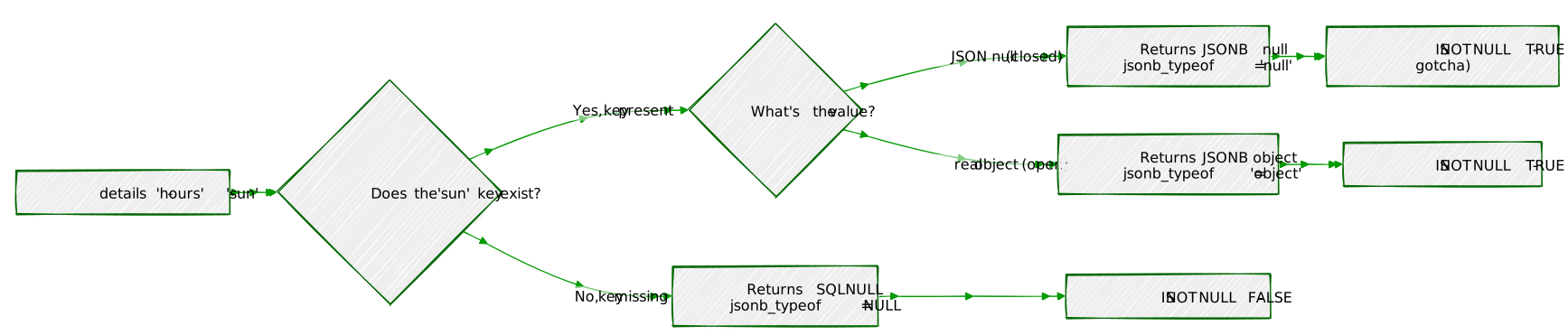
To correctly distinguish the three states, use
jsonb_typeof():
| State | details -> 'hours' -> 'sun' |
jsonb_typeof(...) |
IS NOT NULL |
|---|---|---|---|
| Key missing (accommodation) | SQL NULL |
SQL NULL |
FALSE |
Key present, closed (null) |
JSONB null |
'null' |
TRUE ← gotcha |
| Key present, open (object) | JSONB object | 'object' |
TRUE |
The correct query for “businesses actually open on Sunday”:
SELECT name
FROM   businesses
WHERE  jsonb_typeof(details -> 'hours' -> 'sun') = 'object'
ORDER  BY name;
This returns 25 rows — only the businesses with a
real hours object for Sunday. jsonb_typeof returns
'object' only for JSON objects, 'null' for
JSON null, and SQL NULL for a missing key (which then fails
the = test).
Rule of thumb: Never use
IS NOT NULLto test whether a JSONB navigation result is a “real” value. Usejsonb_typeof(...)to check the actual JSON type, or navigate one level deeper (e.g., checkdetails #>> '{hours,sun,open}') — the#>>operator converts JSON null to SQL NULL, so a deeper path naturally filters it out.
3.2 — Handling accommodation differently
Hotels and hostels store hours as a single
"reception": "HH:MM-HH:MM" string rather than a day-keyed
object. This means the ? 'sun' test returns false for them
even though they may be open 24/7. Write a query that finds all
businesses that are either:
sun),
orSELECT name, neighbourhood,
CASE
WHEN jsonb_typeof(details -> 'hours' -> 'sun') = 'object'
THEN (details #>> '{hours,sun,open}') || '–' ||
(details #>> '{hours,sun,close}')
WHEN details #>> '{hours,reception}' = '24/7'
THEN '24/7'
ELSE details #>> '{hours,reception}'
END AS sunday_availability
FROM businesses
WHERE jsonb_typeof(details -> 'hours' -> 'sun') = 'object'
OR (details -> 'hours') ? 'reception'
ORDER BY neighbourhood, name;Without an index, every JSONB query is a sequential scan — PostgreSQL reads every row and evaluates the expression. For a 48-row toy dataset that is unnoticeable, but with millions of rows it becomes a bottleneck.
A GIN (Generalised Inverted Index) index over a
JSONB column indexes every key and value inside every document. It
accelerates @>, ?, ?|, and
?& queries.
4.1 — Observe the plan before indexing
EXPLAIN (ANALYZE, BUFFERS)
SELECT name
FROM   businesses
WHERE  details @> '{"tags": ["waterfront"]}';
With 48 rows you will see Seq Scan (sequential scan,
i.e. reading every row) — that is expected. On a larger table this would
say Seq Scan with a high cost estimate.
4.2 — Create the GIN index
CREATE INDEX idx_businesses_details_gin
    ON businesses
    USING GIN (details);
4.3 — Observe the plan after indexing
EXPLAIN (ANALYZE, BUFFERS)
SELECT name
FROM   businesses
WHERE  details @> '{"tags": ["waterfront"]}';
On a small table PostgreSQL may still choose a sequential scan (the planner knows the table fits in memory). Force it to use the index to see the mechanism:
SET enable_seqscan = off;

EXPLAIN (ANALYZE, BUFFERS)
SELECT name
FROM   businesses
WHERE  details @> '{"tags": ["waterfront"]}';

SET enable_seqscan = on;   -- always restore this
You should now see
Bitmap Index Scan on idx_businesses_details_gin in the
plan. The GIN index will pay for itself in production as the table
grows.
What GIN indexes: The default
jsonb_opsoperator class indexes every key and value in the document, supporting@>,?,?|,?&. Ajsonb_path_opsclass indexes only values (not keys), producing a smaller index that is faster for@>but cannot accelerate?queries. Usejsonb_path_opswhen you only ever query by value containment and index size matters.
-- Alternative: value-only index (smaller, faster @>, no ? support)
CREATE INDEX idx_businesses_details_pathops
    ON businesses
USING GIN (details jsonb_path_ops);JSONB columns are immutable at the document level — you cannot change a single key without rewriting the whole value. PostgreSQL gives you two tools to do that rewrite concisely.
5.1 — jsonb_set: replace or add one
value
The Lighthouse Bookshop just received a flood of five-star reviews. Update its rating to 5.0:
UPDATE businesses
SET    details = jsonb_set(details, '{rating}', '5.0')
WHERE  name = 'Lighthouse Bookshop';
Verify:
SELECT name, details ->> 'rating' AS rating
FROM   businesses
WHERE  name = 'Lighthouse Bookshop';
jsonb_set(target, path, new_value) — the path is a text
array of keys. If the key already exists it is replaced; if it does not
exist it is added (by default — there is a fourth parameter to suppress
creation).
5.2 — jsonb_set on a nested key
The Gilded Clam is now closing an hour later on Sundays:
UPDATE businesses
SET    details = jsonb_set(
                    details,
                    '{hours,sun,close}',
                    '"21:00"'     -- note: a JSON string must be double-quoted
                )
WHERE  name = 'The Gilded Clam';
SELECT name,
details #>> '{hours,sun,close}' AS new_sunday_close
FROM businesses
WHERE name = 'The Gilded Clam';5.3 — || merge operator: add or overwrite
multiple keys at once
The || operator merges two JSONB objects, with the right
side winning on conflicts. Use it to add a verified flag
and update review_count in a single statement:
UPDATE businesses
SET    details = details || '{"verified": true, "review_count": 999}'
WHERE  name = 'Anchor & Oar Tavern';
SELECT name,
details ->> 'verified' AS verified,
details ->> 'review_count' AS reviews
FROM businesses
WHERE name = 'Anchor & Oar Tavern';Caution:
||does a shallow merge. Ifdetailscontains a nested object likehoursand you merge another object that also hashours, the entirehoursvalue is replaced — not deep-merged. Usejsonb_setfor targeted nested updates.
jsonb_array_elementsThe tags key in most business documents is a JSON array.
To query across tags — for example, to find the most common ones across
the whole directory — you need to expand the array into individual
rows.
6.1 — Expand one business’s tags
SELECT name,
       jsonb_array_elements_text(details -> 'tags') AS tag
FROM   businesses
WHERE  name = 'The Gilded Clam';
name | tag
------------------+---------------
The Gilded Clam | waterfront
The Gilded Clam | seafood
The Gilded Clam | romantic
The Gilded Clam | outdoor_seating
(4 rows)
jsonb_array_elements_textis a set-returning function: each element of the array becomes its own row. The result has more rows than the input.
6.2 — Count tags across all businesses
SELECT tag, COUNT(*) AS occurrences
FROM   businesses,
       jsonb_array_elements_text(details -> 'tags') AS tag
GROUP  BY tag
ORDER  BY occurrences DESC
LIMIT  15;
tag | occurrences
------------------+-------------
waterfront | 10
takeaway | 5
family_friendly | 4
family_owned | 4
organic | 3
...
(15 rows)Your exact numbers will differ — this shows the query pattern. The
comma between businesses and the
jsonb_array_elements_text(...) call is a lateral
join (PostgreSQL expands the function for each input row
automatically when used in the FROM clause this way).
6.3 — Only businesses with multiple specific tags
Find restaurants that are both vegan_options and
takeaway:
SELECT name, details ->> 'cuisine' AS cuisine
FROM   businesses
WHERE  details @> '{"tags": ["vegan_options"]}'
  AND  details @> '{"tags": ["takeaway"]}';
Because each @> call is independent, both conditions
must hold. This is more efficient than expanding the array when the GIN
index is in place.
jsonb_path_queryThe @? operator and jsonb_path_query()
function implement SQL/JSON path language — a
mini-query language for navigating and filtering within a JSONB
document. It is more expressive than chained arrow operators for
conditional navigation.
7.1 — Simple path existence
Find businesses where the social links include Instagram:
SELECT name
FROM   businesses
WHERE  details @? '$.social.instagram';
$.social.instagram means: start at the root
($), descend to social, then to
instagram. @? returns true if the path
resolves to at least one value.
7.2 — Filter on a nested value
Find restaurants with a rating above 4.5:
SELECT name,
       details ->> 'rating' AS rating
FROM   businesses
WHERE  details @? '$ ? (@.category == "restaurant" && @.rating > 4.5)';
name | rating
-----------------------+--------
Bella Napoli | 4.6
Le Petit Bistro | 4.7
River Bend Bakery | 4.8
Spice Garden | 4.6
The Gilded Clam | 4.5
(5 rows)The ? (filter) syntax inside a path expression is
equivalent to a WHERE clause inside the document.
7.3 — Find businesses open late on Friday
Businesses that close at or after 21:00 on Friday (using string
comparison, which works correctly for 24-hour HH:MM
strings):
SELECT name,
       details #>> '{hours,fri,close}' AS friday_close
FROM   businesses
WHERE  details @? '$.hours.fri.close ? (@ >= "21:00")'
ORDER  BY friday_close DESC, name;
name | friday_close
--------------------------+--------------
Bella Napoli | 23:00
Dragon Palace | 23:00
Harbour View Theater | 23:00
The Hungry Scholar | 23:00
Spice Garden | 23:00
Sol y Mar | 23:00
Mango Bay Caribbean | 22:30
The Gilded Clam | 22:30
Thai Orchid | 22:00
The Riverside Vegan | 22:00
Northgate Grocers | 21:00
Lotus Spa & Wellness | 20:00
(12 rows)Limitation to notice: Businesses that close after midnight — Anchor & Oar, The Clocktower Pub, The Rusty Anchor, and others — show a
closeof"01:00"or"02:00". Lexicographically,"02:00" < "21:00", so these businesses are excluded from the above results even though they are open very late. This is a design trade-off of storing times as plain strings. One solution is to store closing times past midnight as"25:00","26:00", etc. — an unusual but practical convention for 24-hour time arithmetic.
7.4 — Extract values with
jsonb_path_query
@? is a boolean test. jsonb_path_query()
returns the actual matched values:
SELECT name,
       jsonb_path_query(details, '$.hours.fri.close') AS friday_close_json
FROM   businesses
WHERE  details @? '$.hours.fri'
ORDER  BY name
LIMIT  8;
The returned values are JSONB (note the quotes around the time
strings). Use jsonb_path_query_first(...) #>> '{}' to
extract a single scalar as text without the surrounding quotes.
You have worked through the core JSONB toolkit. Here is what each operator and function you used actually does:
| Tool | What it does |
|---|---|
-> 'key' |
Navigate one level; returns JSONB |
->> 'key' |
Navigate one level; returns text |
#>> '{a,b,c}' |
Navigate a path; returns text; JSON null becomes SQL NULL |
@> '{"k":"v"}' |
Containment test; accelerated by GIN |
? 'key' |
Key exists test (regardless of value); accelerated by GIN |
?| / ?& |
Any-key / all-keys exist; accelerated by GIN |
jsonb_typeof(val) |
Returns 'object', 'array',
'string', 'number', 'boolean', or
'null'; SQL NULL for a missing key |
jsonb_set(col, path, val) |
Replace or insert a nested value |
col \|\| '{"k":"v"}' |
Shallow-merge a document |
jsonb_array_elements_text(col) |
Expand a JSON array into rows |
@? 'path' |
SQL/JSON path existence test |
jsonb_path_query(col, 'path') |
SQL/JSON path — return matched values |
Remember: JSONB
null≠ SQLNULL. Usejsonb_typeof()— notIS NOT NULL— when you need to distinguish a missing key from a key that exists but holds a JSON null value.
The key design insight from this chapter is that
JSONB lets you keep a relational spine — the columns your queries always
need (id, name, neighbourhood) —
while storing everything else in a document whose shape can vary row by
row. The GIN index means you do not pay a query performance penalty for
that flexibility.
In the next chapter you will add point geometry to the
businesses table and use PostGIS to answer spatial
questions: which businesses are within 500 metres of the harbour, and
which neighbourhood does each one belong to.
Going further: PostgreSQL 14+ supports the jsonpath
type natively. The jsonb_path_query_array and
jsonb_path_query_first variants are useful for pagination
and single-value extraction. For write-heavy workloads, profile whether
JSONB or a computed stored column (Chapter 16) gives better
INSERT/UPDATE throughput on your
hardware.
“A city is not a list of rows. It is a shape on the ground.”
Every interesting question about a city is ultimately a spatial question. Which businesses are near the harbour? Which neighbourhood is this address in? How large is the industrial waterfront? Relational databases answer these badly when location is stored as a text field or a pair of float columns — there is no native concept of “within”, “contains”, or “distance”.
PostGIS is a PostgreSQL extension that adds first-class geometry and geography types, plus several hundred spatial functions and operators. It turns PostgreSQL into a full spatial database: you can store points, lines, and polygons; index them with GIST; and answer proximity, containment, and area queries in SQL without an external GIS system.
This matters in practice far beyond mapping applications. Address geocoding, logistics routing, fraud detection (is this login coming from the expected region?), real estate valuation, and urban planning all reach for spatial queries. PostGIS is the standard tool for all of them in the PostgreSQL ecosystem.
The Portsmith business directory from Chapter 1 stores each business’s neighbourhood as a plain text column. That works for simple filtering, but it cannot answer where questions: it cannot find businesses near a given coordinate, cannot verify that a business address actually falls inside its declared neighbourhood, and cannot measure distances.
This chapter adds a point geometry to every business record, then introduces three new spatial tables:
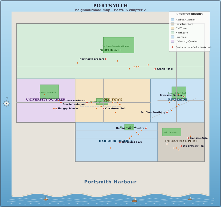
Portsmith’s six neighbourhoods, parks, and featured businesses —
rendered directly from this chapter’s own neighborhoods,
parks, and businesses tables via
utils/render_map.py. Every shape and dot on this map is a
row you’re about to query.
| Table | Geometry type | What it holds |
|---|---|---|
neighborhoods |
POLYGON |
Boundary polygons for Portsmith’s six neighbourhoods |
parks |
POLYGON |
Six public parks and green spaces |
city_infrastructure |
LINESTRING |
Twelve named road segments |
All coordinates are in WGS-84 (SRID 4326), the same coordinate system used by GPS and most web mapping APIs.
By the end of this chapter you will be able to:
POLYGON geometry using WKT
(Well-Known Text) and ST_GeomFromText.ST_DWithin, and understand
why the ::geography cast matters for distance
accuracy.ST_Within and
ST_Contains, and explain the difference between them.ST_Area with the geography type.ST_Distance and a CROSS JOIN LATERAL.PostGIS is a separate package from PostgreSQL. On Debian/Ubuntu:
sudo apt install -y postgresql-16-postgis-3Connect to the portsmith database and enable the
extension:
psql portsmithCREATE EXTENSION IF NOT EXISTS postgis;Verify it loaded:
SELECT postgis_full_version();You should see a long string beginning with
POSTGIS="3.x.x". If you see an error about the extension
not existing, the server package is not installed.
Chapter 1’s seed script must have been run first — the
businesses table must exist. If it does not:
python data/ch01_seed.pypython data/ch02_seed.pyExpected output:
Connecting to: dbname=portsmith
Enabling PostGIS extension …
Applying DDL …
Inserting 6 neighbourhoods …
Inserting 6 parks …
Inserting 12 road segments …
Updating 48 business locations …

Done:
  businesses with geometry : 48
  neighbourhoods           : 6
  parks                    : 6
road segments : 12Open psql portsmith and run these four checks.
Check 1 — businesses now has a geometry column:
\d businessesYou should see a new geom column of type
geometry(Point,4326).
Check 2 — neighbourhood table structure and row count:
SELECT name, population,
       ST_AsText(geom) AS wkt_preview
FROM   neighborhoods
ORDER  BY name;
name | population | wkt_preview
--------------------+------------+------------------------------------
Harbour District | 4200 | POLYGON((-1.805 50.69,...))
Industrial Port | 2100 | POLYGON((-1.77 50.69,...))
Northgate | 18500 | POLYGON((-1.83 50.732,...))
Old Town | 6800 | POLYGON((-1.805 50.71,...))
Riverside | 9300 | POLYGON((-1.773 50.71,...))
University Quarter | 11200 | POLYGON((-1.83 50.71,...))
(6 rows)Check 3 — parks and roads:
SELECT COUNT(*) FROM parks;
SELECT COUNT(*) FROM city_infrastructure;
Both should return 6 and 12 respectively.
Check 4 — SRID on all tables:
SELECT f_table_name, f_geometry_column, srid, type
FROM   geometry_columns
WHERE  f_table_schema = 'public'
ORDER  BY f_table_name;
f_table_name | f_geometry_column | srid | type
------------------------+-------------------+------+------------
businesses | geom | 4326 | POINT
city_infrastructure | geom | 4326 | LINESTRING
neighborhoods | geom | 4326 | POLYGON
parks | geom | 4326 | POLYGON
(4 rows)If all four pass, proceed to the exercises.
Geometry in PostGIS is often loaded from Well-Known Text (WKT), a human-readable representation of shapes. Understanding WKT lets you read geometry from SQL output, write it in queries, and reason about what you stored.
1.1 — Read a polygon in WKT
SELECT name, ST_AsText(geom) AS wkt
FROM   neighborhoods
WHERE  name = 'Harbour District';
name | wkt
-------------------+------------------------------------------------------
Harbour District | POLYGON((-1.805 50.69,-1.77 50.69,-1.77 50.71,...))WKT for a polygon is POLYGON((x1 y1, x2 y2, ...)). In
geographic coordinates the convention is longitude latitude (x
then y), matching the X/Y convention in maths. The ring must
close — the last coordinate must equal the first.
1.2 — Inspect the bounding box
ST_Envelope returns the minimum bounding rectangle for
any geometry:
SELECT name,
       ST_XMin(ST_Envelope(geom)) AS west,
       ST_XMax(ST_Envelope(geom)) AS east,
       ST_YMin(ST_Envelope(geom)) AS south,
       ST_YMax(ST_Envelope(geom)) AS north
FROM   neighborhoods
ORDER  BY name;
Use this output to confirm each polygon sits in the right part of the coordinate space (longitudes around −1.75 to −1.83, latitudes around 50.69 to 50.76).
1.3 — Count vertices
SELECT name,
       ST_NPoints(geom) AS vertex_count
FROM   neighborhoods
ORDER  BY name;
Each neighbourhood polygon has five vertices (four corners plus the closing duplicate). A real city boundary imported from an OS/census shapefile might have thousands.
1.4 — Understand the SRID
ST_SRID returns the spatial reference identifier stored
with the geometry:
SELECT name, ST_SRID(geom) AS srid
FROM   neighborhoods
LIMIT  3;
SRID 4326 is the WGS-84 system used by GPS. Every geometry in these tables carries the same SRID, which means they can be compared and joined directly. If SRIDs differ, PostGIS will return an error — a deliberate safety check.
The geometry/geography distinction: In PostGIS,
geometrystores coordinates in whatever units the SRS defines. For SRID 4326 that means degrees. When you ask for a distance between twogeometrypoints in 4326, you get a value in degrees — nearly useless for human-scale distances. Thegeographytype, by contrast, always works on a spheroid and returns distances in metres. You can cast any SRID-4326 geometry to geography with::geographyto get metre-based calculations. The exercises use this cast throughout.
ST_DWithinST_DWithin(a, b, distance) returns true when the
distance between a and b is at most
distance. With geography inputs the distance is in
metres.
2.1 — Find businesses within 500 m of Portsmith Pier
Portsmith’s main pier entrance sits at approximately (−1.785, 50.700). Find every business within 500 metres of it:
SELECT b.name,
       b.neighbourhood,
       ROUND(
           ST_Distance(b.geom::geography,
                       ST_Point(-1.785, 50.700)::geography)::numeric
       ) AS distance_m
FROM   businesses b
WHERE  ST_DWithin(b.geom::geography,
                  ST_Point(-1.785, 50.700)::geography,
                  500)
ORDER  BY distance_m;
name | neighbourhood | distance_m
-------------------------+------------------+------------
The Gilded Clam | Harbour District | 70
Anchor & Oar Tavern | Harbour District | 179
Tidal Wave Surf Shop | Harbour District | 307
Harbour Inn | Harbour District | 437
Portsmith Fish Market | Harbour District | 484
(5 rows)All five results are in the Harbour District — exactly what you would expect for a search centred on the pier.
2.2 — Why ::geography matters
Try the same query without the cast. Note that
ST_Point(...) without an explicit SRID gets SRID 0, which
PostGIS refuses to compare against SRID-4326 geometry — so you must use
ST_SetSRID:
SELECT b.name,
       ROUND(ST_Distance(b.geom,
                         ST_SetSRID(ST_Point(-1.785, 50.700), 4326))::numeric,
             6)                AS distance_degrees
FROM   businesses b
WHERE  ST_DWithin(b.geom,
                  ST_SetSRID(ST_Point(-1.785, 50.700), 4326),
                  500)
ORDER  BY distance_degrees;
The WHERE clause now has a threshold of 500
— but in degrees. One degree of latitude is about 111 km, so
this matches businesses within roughly 55,000 km: all 48 of them, from
the whole city. The distance_degrees values in the output
are tiny fractions like 0.001000, not useful numbers.
rows returned: 48 (the entire city, not 5)Rule: For any distance query on SRID-4326 data, always cast to
::geographyinST_DWithinandST_Distance. The cast has negligible performance cost at the scales used in city-level data.
2.3 — Try different radii
How many businesses fall within 1 km of the pier? 2 km?
SELECT radius_m,
       COUNT(*) AS business_count
FROM   (VALUES (500), (1000), (2000)) AS radii(radius_m)
CROSS JOIN LATERAL (
    SELECT 1
    FROM   businesses b
    WHERE  ST_DWithin(b.geom::geography,
                      ST_Point(-1.785, 50.700)::geography,
                      radius_m)
) AS matches
GROUP  BY radius_m
ORDER  BY radius_m;
radius_m | business_count
----------+----------------
500 | 5
1000 | 8
2000 | 17
(3 rows)The pier sits in the southern Harbour District. Doubling the radius to 2 km pulls in more of the central neighbourhoods, but the northern Northgate businesses are nearly 5 km away — a reminder that Portsmith stretches a significant distance north from the waterfront.
ST_Within and
ST_ContainsA spatial join links rows from two tables based on a geometric relationship rather than a key match. The most common are containment tests: does point A fall inside polygon B?
3.1 — Which neighbourhood is each business in?
SELECT b.name,
       b.neighbourhood          AS declared_neighbourhood,
       n.name                   AS postgis_neighbourhood
FROM   businesses  b
JOIN   neighborhoods n ON ST_Within(b.geom, n.geom)
ORDER  BY n.name, b.name;
ST_Within(a, b) returns true when geometry
a lies completely inside geometry b. The query
should return all 48 businesses, each matched to its neighbourhood.
Confirm the declared neighbourhood column always matches
postgis_neighbourhood:
SELECT COUNT(*) AS mismatches
FROM   businesses  b
JOIN   neighborhoods n ON ST_Within(b.geom, n.geom)
WHERE  b.neighbourhood <> n.name;
mismatches
------------
0
(1 row)Zero mismatches: the text column from Chapter 1 and the geometry are consistent.
3.2 — ST_Contains is the inverse
ST_Contains(a, b) returns true when polygon
a contains geometry b — it is the mirror of
ST_Within. These two queries produce identical results:
-- Point inside polygon
SELECT b.name FROM businesses b
JOIN   neighborhoods n ON ST_Within(b.geom, n.geom)
WHERE  n.name = 'Old Town'
ORDER  BY b.name;

-- Polygon contains point
SELECT b.name FROM businesses b
JOIN   neighborhoods n ON ST_Contains(n.geom, b.geom)
WHERE  n.name = 'Old Town'
ORDER  BY b.name;
name
--------------------------
Bella Napoli
Finch & Sons Barbers
Le Petit Bistro
Old Town Hardware
Portsmith Accountancy Ltd.
Portsmith Arms Hotel
Portsmith Legal Group
Portsmith Tailors
The Clocktower Pub
(9 rows)Both return the same 9 Old Town businesses.
The subtle difference:
ST_Contains(A, B)requires that no point of B lies on the boundary of A. A point sitting exactly on a polygon edge would failST_Containsbut passST_Covers. In practice, coordinates rarely land precisely on a boundary, so the two functions behave identically for most point-in-polygon work. Reach forST_Coversif you need to include boundary-touching cases explicitly.
3.3 — Check for gaps: businesses in no neighbourhood
This query finds any businesses whose geometry falls outside every neighbourhood polygon — useful for catching data quality problems:
SELECT b.name, b.neighbourhood
FROM   businesses b
WHERE  NOT EXISTS (
    SELECT 1
    FROM   neighborhoods n
    WHERE  ST_Within(b.geom, n.geom)
);
name | neighbourhood
------+---------------
(0 rows)All 48 businesses are inside a neighbourhood polygon.
ST_Area returns the area of a polygon. Called on
geometry (degrees), it returns a value in square degrees —
meaningless to most people. Called on geography, it returns
square metres.
4.1 — Incorrect: area in square degrees
SELECT name,
       ROUND(ST_Area(geom)::numeric, 6) AS area_sq_degrees
FROM   neighborhoods
ORDER  BY area_sq_degrees DESC;
The numbers look tiny (around 0.0007). They are
geometrically correct but impossible to interpret as real-world area
because degrees are not uniform units.
4.2 — Correct: area in square metres, then kilometres
SELECT name,
       ROUND((ST_Area(geom::geography) / 1e6)::numeric, 2) AS area_km2
FROM   neighborhoods
ORDER  BY area_km2 DESC;
name | area_km2
--------------------+----------
Northgate | 17.59
Old Town | 5.53
Harbour District | 5.50
University Quarter | 4.32
Riverside | 3.98
Industrial Port | 3.14
(6 rows)Northgate is by far the largest neighbourhood — it spans the entire northern width of the city. Industrial Port is the smallest, a tight strip of dockside land. Old Town and Harbour District are almost identical in area despite having very different characters.
Why the numbers differ slightly from manual estimates:
ST_Areaon geography uses the WGS-84 spheroid, which accounts for the fact that the Earth is not a perfect sphere. At latitude 50.7° the correction is small (under 0.3%) but present.
4.3 — Population density
Combine the computed area with the population
column:
SELECT name,
       population,
       ROUND((ST_Area(geom::geography) / 1e6)::numeric, 2) AS area_km2,
       ROUND(
           (population / (ST_Area(geom::geography) / 1e6))::numeric
       ) AS pop_per_km2
FROM   neighborhoods
ORDER  BY pop_per_km2 DESC;
name | population | area_km2 | pop_per_km2
--------------------+------------+----------+-------------
University Quarter | 11200 | 4.32 | 2592
Riverside | 9300 | 3.98 | 2340
Old Town | 6800 | 5.53 | 1230
Northgate | 18500 | 17.59 | 1052
Harbour District | 4200 | 5.50 | 763
Industrial Port | 2100 | 3.14 | 668
(6 rows)The University Quarter and Riverside are the most densely populated neighbourhoods — student housing and riverside apartments pack a lot of people into compact areas. The Industrial Port is the least dense despite its small size; much of it is warehouse and dock rather than residential.
ST_Distance and a Lateral JoinFinding the nearest feature from another table requires a lateral join — a subquery that can reference columns from the outer query row by row.
5.1 — Distance from one business to one park
ST_Distance between two geography values returns
metres:
SELECT b.name                          AS business,
       p.name                          AS park,
       ROUND(ST_Distance(b.geom::geography,
                         p.geom::geography)::numeric) AS distance_m
FROM   businesses b,
       parks p
WHERE  b.name = 'The Gilded Clam'
ORDER  BY distance_m;
business | park | distance_m
------------------+-----------------------------+------------
The Gilded Clam | Harbourside Park | 682
The Gilded Clam | Dockside Green | 1315
The Gilded Clam | Market Square Gardens | 2143
The Gilded Clam | Riverside Walk Park | 2899
The Gilded Clam | University Grounds | 3060
The Gilded Clam | Northgate Recreation Ground | 5006
(6 rows)The nearest park to The Gilded Clam is Harbourside Park, 682 m away.
The ST_Distance to a polygon returns the distance from the
point to the nearest point on the polygon’s boundary — zero when the
point is inside the polygon.
5.2 — Nearest park for a single business (lateral pattern)
The canonical pattern for “nearest one thing” is
ORDER BY ... LIMIT 1 inside a lateral subquery:
SELECT b.name,
       nearest.park_name,
       nearest.distance_m
FROM   businesses b
CROSS JOIN LATERAL (
    SELECT p.name                                               AS park_name,
           ROUND(ST_Distance(b.geom::geography,
                             p.geom::geography)::numeric)      AS distance_m
    FROM   parks p
    ORDER  BY b.geom::geography <-> p.geom::geography
    LIMIT  1
) AS nearest
WHERE  b.name = 'Quarter Note Jazz Club';
name | park_name | distance_m
-----------------------+--------------------+------------
Quarter Note Jazz Club | University Grounds | 233
(1 row)The <-> operator is the KNN (k-nearest-neighbour)
distance operator. When used in an ORDER BY clause inside a
lateral join, PostGIS can accelerate it with the GIST index (which you
will create in Exercise 6). Using <-> in
ORDER BY is preferred over
ORDER BY ST_Distance(...) for this reason.
5.3 — Nearest park for every business
Remove the WHERE filter to run across all 48
businesses:
SELECT b.name                          AS business,
       b.neighbourhood,
       nearest.park_name,
       nearest.distance_m
FROM   businesses b
CROSS JOIN LATERAL (
    SELECT p.name                                               AS park_name,
           ROUND(ST_Distance(b.geom::geography,
                             p.geom::geography)::numeric)      AS distance_m
    FROM   parks p
    ORDER  BY b.geom::geography <-> p.geom::geography
    LIMIT  1
) AS nearest
ORDER  BY b.neighbourhood, b.name;
Scan the results. You should see a clean pattern: each
neighbourhood’s businesses point to the park in that same neighbourhood.
Notice that three Riverside businesses (Portsmith Pharmacy, Portsmith
Veterinary Clinic, Riverside Cinema) and University Bookshop all show
distance_m = 0 — their coordinates fall inside the
park polygon. ST_Distance to a polygon returns zero when
the point is contained within it.
5.4 — Aggregate: average walking distance to a park, by neighbourhood
SELECT b.neighbourhood,
       ROUND(AVG(nearest.distance_m)::numeric) AS avg_distance_m
FROM   businesses b
CROSS JOIN LATERAL (
    SELECT ROUND(ST_Distance(b.geom::geography,
                             p.geom::geography)::numeric) AS distance_m
    FROM   parks p
    ORDER  BY b.geom::geography <-> p.geom::geography
    LIMIT  1
) AS nearest
GROUP  BY b.neighbourhood
ORDER  BY avg_distance_m;
This gives a rough “walkability to green space” metric per neighbourhood. Old Town ranks first — Market Square Gardens sits centrally within the neighbourhood. Northgate comes last despite having the largest park, because the park is in the far north of the district while businesses cluster near the southern edge.
Without an index, every spatial query is a sequential scan: PostgreSQL reads every row, applies the geometry function, and discards non-matching rows. For a 48-row dataset that is instant, but at 48 million rows it is not.
PostGIS spatial queries are accelerated by GIST (Generalised Search Tree) indexes. A GIST index on a geometry column builds a tree of bounding boxes, allowing the planner to quickly eliminate large portions of the table.
6.1 — Observe the plan before indexing
EXPLAIN (ANALYZE, BUFFERS)
SELECT name
FROM   businesses
WHERE  ST_DWithin(geom::geography,
                  ST_Point(-1.785, 50.700)::geography,
                  500);
On the 48-row businesses table you will see something
like:
Seq Scan on businesses  (cost=0.00..4.60 rows=1 width=...) ...
  Filter: (st_dwithin(...))
  Rows Removed by Filter: 43
A sequential scan is expected on a tiny table — the planner knows the overhead of an index lookup exceeds the cost of reading all 48 rows.
6.2 — Create GIST indexes on the geometry columns
CREATE INDEX idx_businesses_geom
    ON businesses USING GIST (geom);

CREATE INDEX idx_neighborhoods_geom
    ON neighborhoods USING GIST (geom);

CREATE INDEX idx_parks_geom
    ON parks USING GIST (geom);

CREATE INDEX idx_city_infrastructure_geom
    ON city_infrastructure USING GIST (geom);
6.3 — The geometry/geography index split
With enable_seqscan off, verify which plan the proximity
query uses:
SET enable_seqscan = off;

EXPLAIN (ANALYZE, BUFFERS)
SELECT name
FROM   businesses
WHERE  ST_DWithin(geom::geography,
                  ST_Point(-1.785, 50.700)::geography,
                  500);

SET enable_seqscan = on;
You will see — perhaps surprisingly — that the planner still
uses a sequential scan, even though idx_businesses_geom
exists:
Seq Scan on businesses  (cost=10000000000.00...) ...
  Filter: st_dwithin((geom)::geography, ...)
Why? The GIST index was built on geom
(type geometry). The query filters on
geom::geography (type geography). These are
different types — the index is not usable for geography operations.
To accelerate geography-based distance queries you need a functional index on the cast:
CREATE INDEX idx_businesses_geom_geography
    ON businesses USING GIST (CAST(geom AS geography));
Now with enable_seqscan off:
SET enable_seqscan = off;

EXPLAIN (ANALYZE, BUFFERS)
SELECT name
FROM   businesses
WHERE  ST_DWithin(geom::geography,
                  ST_Point(-1.785, 50.700)::geography,
                  500);

SET enable_seqscan = on;
Index Scan using idx_businesses_geom_geography on businesses
Index Cond: ((geom)::geography &&
_st_expand('...', '500'))
Filter: st_dwithin((geom)::geography, ...)
Rows Removed by Filter: 2The index is now used. The index condition uses
&& (bounding-box overlap on the spheroid) to
quickly discard most rows, then st_dwithin rechecks the
exact distance for the survivors.
6.4 — Verify the spatial join plan
The containment join uses geometry-to-geometry operations, so
idx_businesses_geom (the plain geometry index) is
used there:
SET enable_seqscan = off;

EXPLAIN (ANALYZE, BUFFERS)
SELECT b.name, n.name AS neighbourhood
FROM   businesses b
JOIN   neighborhoods n ON ST_Within(b.geom, n.geom);

SET enable_seqscan = on;
Nested Loop ...
-> Seq Scan on neighborhoods n (6 rows — tiny table)
-> Index Scan using idx_businesses_geom on businesses b
Index Cond: (geom @ n.geom)
Filter: st_within(geom, n.geom)For each neighbourhood polygon, idx_businesses_geom is
used to find businesses whose bounding box falls inside the
neighbourhood’s bounding box (geom @ n.geom), then
st_within rechecks the exact containment.
The index rule: A GIST index on
geom geometryaccelerates geometry-to-geometry operations (ST_Within,ST_Contains,ST_Intersects,&&). A GIST index onCAST(geom AS geography)accelerates geography operations (ST_DWithin(...::geography, ...),<->on geography). If you query both ways, create both indexes — they coexist happily on the same table.
You have worked through the core PostGIS toolkit for points, polygons, and linear features. Here is a reference for everything used:
| Function / operator | What it does |
|---|---|
ST_GeomFromText(wkt, srid) |
Parse WKT into a geometry with the given SRID |
ST_AsText(geom) |
Format geometry as WKT for display |
ST_SetSRID(ST_MakePoint(lon, lat), srid) |
Construct a point geometry |
ST_Point(lon, lat)::geography |
Construct a point and cast to geography |
geom::geography |
Cast a 4326 geometry to geography (distances now in metres) |
ST_SRID(geom) |
Return the SRID stored with a geometry |
ST_NPoints(geom) |
Count vertices in a geometry |
ST_Envelope(geom) |
Return the bounding-box rectangle |
ST_XMin/XMax/YMin/YMax(geom) |
Extract bounding-box extents |
ST_DWithin(a, b, d) |
True when the distance between a and b is ≤ d |
ST_Distance(a, b) |
Distance between two geometries (metres for geography) |
a::geography <-> b::geography |
KNN distance operator; use in ORDER BY for index acceleration |
ST_Within(a, b) |
True when a lies completely inside b |
ST_Contains(a, b) |
True when a contains b (inverse of ST_Within) |
ST_Area(geom::geography) |
Area in square metres on the spheroid |
CROSS JOIN LATERAL (... LIMIT 1) |
Nearest-neighbour join pattern |
USING GIST (geom) |
Create a GIST spatial index |
Geometry vs geography in one sentence: Use
geometryfor storage and when working with projected coordinate systems where units are already metres or feet. Cast togeographyany time you need distance, area, or proximity results in real-world units from SRID-4326 data.
The coordinates added in this chapter will carry forward. Chapter 12
extends the city_infrastructure road network into a graph
and uses a recursive CTE to find the shortest path between two
intersections.
Going further: PostGIS supports many more geometry types —
MULTIPOLYGON for areas with holes,
GEOMETRYCOLLECTION for mixed types, and 3D geometries with
a Z coordinate for elevation data. For routing specifically,
pgRouting builds on PostGIS to provide Dijkstra, A*, and
turn-restriction-aware shortest-path algorithms over road network
graphs. For importing real boundary data, shp2pgsql
converts ESRI Shapefiles directly into PostGIS-compatible
INSERT statements, and ogr2ogr handles
GeoJSON, KML, GeoPackage, and dozens of other formats.
FOR UPDATE SKIP LOCKED“A queue is just a table that everyone is racing to read.”
Sooner or later almost every application needs a queue: a list of work items that a pool of workers processes one at a time, safely, without two workers ever grabbing the same item. The reflexive answer is to reach for a message broker — Redis, RabbitMQ, SQS, Kafka. Those tools earn their keep at serious scale. But if your data already lives in PostgreSQL, running a second system just to hand out rows to workers is often unnecessary complexity: another service to deploy, monitor, and keep consistent with the database.
PostgreSQL can do this job itself. The
FOR UPDATE SKIP LOCKED row-locking clause, combined with an
ordinary table, gives you an atomic “claim the next item and don’t let
anyone else touch it” primitive — the same guarantee a dedicated queue
product sells you, built out of two SQL keywords. This chapter builds a
job queue from scratch: the schema, the atomic claim query, concurrent
worker behaviour, stalled-job recovery, and a dead-letter path for jobs
that keep failing.
This is not a toy exercise. This exact pattern — a status column, a
claim query, a heartbeat, a dead-letter table — is what libraries like
river, oban (Elixir),
and countless in-house job runners implement on top of PostgreSQL in
production.
Portsmith’s permitting office processes a steady stream of permit applications: building work, business licenses, public events, signage, and demolitions. Each application needs to move through a review pipeline, and the office wants that processing to happen asynchronously and reliably — work should never be lost, never double-processed, and a crashed reviewer process shouldn’t leave an application stuck in limbo forever.
The jobs table models this as a queue. Every row is one
permit application awaiting review. A status column tracks
its life cycle, a priority column lets safety-critical work
(demolitions) jump ahead of routine work (sign permits), and a retry
counter with a companion dead_letter_jobs table handles
applications whose processing keeps failing.
| Column | Purpose |
|---|---|
status |
queued → in_progress →
completed (or back to queued, or
dead-lettered) |
priority |
1 (most urgent — demolitions) to 5 (least urgent — sign permits) |
payload |
JSONB — the permit application details |
attempts / max_attempts |
Retry bookkeeping |
claimed_by / claimed_at |
Which worker has the job, and since when |
heartbeat_at |
Updated periodically by the worker while it holds the job |
The status column’s life cycle, drawn out — this is what
Exercises 2 through 5 each implement one piece of:
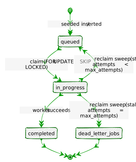
Every arrow here is a specific query you’ll write by hand later in
this chapter — there’s no hidden state machine enforcing this, just the
status column, the claim query, and the reclaim sweep
agreeing on what each value means.
No extensions are required for this chapter — everything here is built on core PostgreSQL locking semantics.
By the end of this chapter you will be able to:
UPDATE ... FROM (SELECT ... FOR UPDATE SKIP LOCKED) claim
query, and explain why naive two-step approaches race.psql sessions, that
SKIP LOCKED lets workers proceed past rows another worker
is holding — and contrast that with the blocking behaviour of plain
FOR UPDATE.pgbench.This chapter needs nothing beyond what Chapter 1 already set up:
PostgreSQL 16 and a Python 3.12 virtual environment with
psycopg. If you skipped Chapter 1, see its Installation
section. You will also use pgbench for Exercise 6, which
ships with the standard PostgreSQL client tools
(postgresql-client-16 on Debian/Ubuntu).
From the book/ directory, with the virtual environment
active:
python data/ch03_seed.pyExpected output:
Connecting to: dbname=portsmith
Creating schema …
Inserting 45 jobs …
Done — 45 rows in jobs, all queued.
The seed script is self-contained — it does not depend on Chapter 1 or 2’s data.
Open psql portsmith and run these checks.
Check 1 — table structure:
\d jobs Table "public.jobs"
Column | Type | Collation | Nullable | Default
--------------+--------------------------+-----------+----------+----------------------------------
id | bigint | | not null | nextval('jobs_id_seq'::regclass)
job_type | text | | not null |
payload | jsonb | | not null |
status | text | | not null | 'queued'::text
priority | smallint | | not null | 5
attempts | integer | | not null | 0
max_attempts | integer | | not null | 3
created_at | timestamp with time zone | | not null | clock_timestamp()
claimed_at | timestamp with time zone | | |
claimed_by | text | | |
heartbeat_at | timestamp with time zone | | |
completed_at | timestamp with time zone | | |
last_error | text | | |
Indexes:
"jobs_pkey" PRIMARY KEY, btree (id)
"idx_jobs_claim_order" btree (priority, created_at, id) WHERE status = 'queued'::text
"idx_jobs_status" btree (status)
Check constraints:
"jobs_status_check" CHECK (status = ANY (ARRAY['queued'::text, 'in_progress'::text, 'completed'::text, 'failed'::text]))Check 2 — job counts by type and priority:
SELECT job_type, priority, COUNT(*) AS jobs
FROM   jobs
GROUP  BY job_type, priority
ORDER  BY priority;
job_type | priority | jobs
-------------------+----------+------
demolition_permit | 1 | 4
business_license | 2 | 12
building_permit | 3 | 15
event_permit | 4 | 8
sign_permit | 5 | 6
(5 rows)Check 3 — everything starts queued:
SELECT status, COUNT(*) FROM jobs GROUP BY status; status | count
--------+-------
queued | 45
(1 row)If all three match, proceed to the exercises.
Note: If you re-run
ch03_seed.pyat any point during the exercises to reset to a clean state, it drops and recreates bothjobsanddead_letter_jobs.
1.1 — Why a partial index
The claim query (which you’ll write in Exercise 2) only ever looks at
rows where status = 'queued', ordered by
priority then created_at. As the queue runs,
the vast majority of rows will end up completed — a normal
B-tree index on (priority, created_at, id) would faithfully
index every one of those settled rows even though the claim query never
looks at them.
idx_jobs_claim_order is a partial index
— it only indexes rows matching
WHERE status = 'queued':
CREATE INDEX idx_jobs_claim_order
    ON jobs (priority, created_at, id)
    WHERE status = 'queued';
This keeps the index small regardless of how many historical jobs
pile up in completed or failed state, because
settled rows are never in it.
1.2 — Why id is part of the sort key, not just
created_at
You might expect ORDER BY priority, created_at to be
enough — oldest job in the highest-priority bucket goes first. But
timestamps are not always unique. If two jobs are inserted in the same
transaction, both can get an identical created_at (more on
this below), and ORDER BY over tied values has no defined
order. Appending the primary key, id, as a final tiebreaker
guarantees a deterministic order even when timestamps collide:
ORDER BY priority ASC, created_at ASC, id ASCA gotcha worth knowing:
now()returns the transaction’s start time, not the current wall-clock time — every call tonow()inside the same transaction returns the same value. The seed script originally usedcreated_at TIMESTAMPTZ DEFAULT now(), and because all 45 rows were inserted in one transaction, every single row ended up with an identicalcreated_at. The fix isclock_timestamp(), which returns the actual current time at the moment it’s evaluated, differing row to row even within one transaction.jobs.created_atusesclock_timestamp()for exactly this reason. This is the same family of surprise as the JSONBnullvs. SQLNULLgotcha from Chapter 1: a function name that looks interchangeable with another is not.
1.3 — Confirm the index is used
EXPLAIN (ANALYZE, BUFFERS)
SELECT id
FROM   jobs
WHERE  status = 'queued'
ORDER  BY priority ASC, created_at ASC, id ASC
FOR UPDATE SKIP LOCKED
LIMIT  1;
Limit (cost=0.14..6.17 rows=1 width=24) (actual time=0.022..0.022 rows=1 loops=1)
Buffers: shared hit=3
-> LockRows (cost=0.14..12.20 rows=2 width=24) (actual time=0.021..0.021 rows=1 loops=1)
Buffers: shared hit=3
-> Index Scan using idx_jobs_claim_order on jobs (cost=0.14..12.18 rows=2 width=24) (actual time=0.010..0.010 rows=1 loops=1)
Filter: (status = 'queued'::text)
Buffers: shared hit=2Now drop the index and run the identical query again inside a transaction you roll back (so the drop doesn’t stick):
BEGIN;
DROP INDEX idx_jobs_claim_order;

EXPLAIN (ANALYZE, BUFFERS)
SELECT id
FROM   jobs
WHERE  status = 'queued'
ORDER  BY priority ASC, created_at ASC, id ASC
FOR UPDATE SKIP LOCKED
LIMIT  1;

ROLLBACK;
Limit (cost=9.51..9.53 rows=1 width=24) (actual time=0.071..0.072 rows=1 loops=1)
-> LockRows (cost=9.51..9.54 rows=2 width=24) (actual time=0.070..0.071 rows=1 loops=1)
-> Sort (cost=9.51..9.52 rows=2 width=24) (actual time=0.067..0.068 rows=1 loops=1)
Sort Key: priority, created_at, id
Sort Method: quicksort Memory: 27kB
-> Bitmap Heap Scan on jobs (cost=4.16..9.50 rows=2 width=24) (actual time=0.018..0.027 rows=45 loops=1)
Recheck Cond: (status = 'queued'::text)
-> Bitmap Index Scan on idx_jobs_status (cost=0.00..4.16 rows=2 width=0) (actual time=0.013..0.013 rows=45 loops=1)
Index Cond: (status = 'queued'::text)Without idx_jobs_claim_order, PostgreSQL still finds the
queued rows (via idx_jobs_status), but it must then
sort all of them to find the one with the lowest
(priority, created_at, id) — an extra Sort
node. With the tailored partial index, the rows are already stored in
claim order, so PostgreSQL walks the index and stops at the first match.
On a 45-row table the difference is invisible; on a busy production
queue with a deep backlog, eliminating the sort on every single claim
matters a great deal.
2.1 — Why a naive two-step claim races
The tempting first approach is to SELECT a candidate
row, then UPDATE it in a second statement:
-- ⚠ Do not do this — it has a race condition
SELECT id FROM jobs WHERE status = 'queued' ORDER BY priority, created_at, id LIMIT 1;
-- ... application reads id = 7 ...
UPDATE jobs SET status = 'in_progress' WHERE id = 7;
Between the SELECT and the UPDATE, nothing
stops a second worker from running the exact same SELECT,
reading the same id = 7, and also issuing the
UPDATE. Both workers now believe they own job 7. This is a
classic check-then-act race condition — the gap between
reading and acting is exactly where two workers can interleave.
2.2 — FOR UPDATE closes the gap, but
blocks
Locking the row as part of the SELECT closes the
race:
SELECT id FROM jobs WHERE status = 'queued' ORDER BY priority, created_at, id
FOR UPDATE LIMIT 1;
Now a second worker running the same query, in a separate transaction, blocks until the first worker’s transaction commits or rolls back — correct, but it means every worker but one sits idle waiting for a lock instead of moving on to a different job. Section 3.1 demonstrates this.
2.3 — SKIP LOCKED lets workers move past each
other
Adding SKIP LOCKED tells PostgreSQL: if the next
candidate row is already locked by another transaction, don’t wait for
it — skip it and consider the row after it.
SELECT id FROM jobs WHERE status = 'queued' ORDER BY priority, created_at, id
FOR UPDATE SKIP LOCKED LIMIT 1;
This is the piece that makes PostgreSQL usable as a concurrent queue: N workers can run this query at the same instant and each will walk away with a different row, with no blocking and no double-claims.
2.4 — The full atomic claim: lock, update, and return in one statement
Locking the row is only half the job — you still need to mark it
in_progress before releasing the lock, and you want the
whole thing to happen as a single round trip. Combine the
SELECT ... FOR UPDATE SKIP LOCKED with the
UPDATE using a CTE:
WITH next_job AS (
    SELECT id
    FROM   jobs
    WHERE  status = 'queued'
    ORDER  BY priority ASC, created_at ASC, id ASC
    FOR UPDATE SKIP LOCKED
    LIMIT  1
)
UPDATE jobs
SET    status       = 'in_progress',
       claimed_at   = now(),
       claimed_by   = 'demo-worker',
       heartbeat_at = now(),
       attempts     = attempts + 1
FROM   next_job
WHERE  jobs.id = next_job.id
RETURNING jobs.id, jobs.job_type, jobs.payload ->> 'application_id' AS application_id,
          jobs.priority, jobs.attempts, jobs.status;
id | job_type | application_id | priority | attempts | status
----+-------------------+----------------+----------+----------+-------------
1 | demolition_permit | DP-2024-0001 | 1 | 1 | in_progress
(1 row)This single statement is the entire claim operation: find the best
candidate, skip anything locked, mark it claimed, and hand back its data
— atomically, with no window for a race. This is exactly the query
data/ch03_worker.py runs (see CLAIM_SQL). Run
it again and the demolition permit at id = 2 comes back
next — id = 1 is now in_progress, so it’s no
longer a candidate.
Roll this back if you ran it directly in
psqland want to keep the queue clean for later exercises: wrap it inBEGIN; ... ROLLBACK;.
3.1 — SKIP LOCKED vs. plain
FOR UPDATE, in two psql sessions
Open two terminals with psql portsmith in each. In
Session A, start a transaction, claim 5 rows, and hold
the transaction open (don’t commit yet):
-- Session A
BEGIN;
SELECT id, job_type FROM jobs WHERE status = 'queued'
ORDER BY priority, created_at, id
FOR UPDATE SKIP LOCKED LIMIT 5;
id | job_type
----+-------------------
1 | demolition_permit
2 | demolition_permit
3 | demolition_permit
4 | demolition_permit
5 | business_license
(5 rows)Leave that transaction open. In Session B, run the identical query:
-- Session B (Session A is still open, holding locks on ids 1-5)
BEGIN;
SELECT id, job_type FROM jobs WHERE status = 'queued'
ORDER BY priority, created_at, id
FOR UPDATE SKIP LOCKED LIMIT 5; id | job_type
----+------------------
6 | business_license
7 | business_license
8 | business_license
9 | business_license
10 | business_license
(5 rows)Session B returns immediately with a different set
of rows — it silently skipped 1–5 because they
were locked, and moved on to the next five unlocked candidates. Commit
or roll back both sessions to release the locks:
COMMIT; -- run in both sessions3.2 — Now try it with plain FOR UPDATE (no
SKIP LOCKED)
Repeat the same two-session experiment, but drop
SKIP LOCKED:
-- Session A
BEGIN;
SELECT id, job_type FROM jobs WHERE status = 'queued'
ORDER BY priority, created_at, id
FOR UPDATE LIMIT 5;
-- (leave this transaction open)-- Session B — this will hang
BEGIN;
SELECT id, job_type FROM jobs WHERE status = 'queued'
ORDER BY priority, created_at, id
FOR UPDATE LIMIT 5;Session B does not return. It is blocked, waiting for Session A’s row
locks to be released. Only once Session A runs COMMIT (or
ROLLBACK) does Session B’s query complete — and when it
does, it returns the same five rows Session A had, now that
they’re unlocked again:
-- (Session B, after Session A commits)
 id |     job_type
----+-------------------
  1 | demolition_permit
  2 | demolition_permit
  3 | demolition_permit
  4 | demolition_permit
  5 | business_license
(5 rows)This is the difference in one sentence: plain
FOR UPDATE serializes workers through the lock;
SKIP LOCKED lets them fan out across the table.
For a job queue, you always want the latter — a blocked worker is a
wasted worker. Both runs side by side, as a timeline:
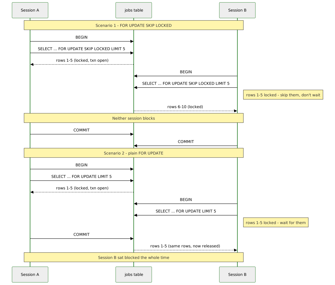
3.3 — Real concurrent workers with
ch03_worker.py
Reset the data (python data/ch03_seed.py) if you ran the
manual claim in Exercise 2.4 without rolling it back. Then launch two
workers in the background, each capped to 10 jobs so they finish
quickly:
python data/ch03_worker.py --worker-id w1 --max-jobs 10 --fail-rate 0 &
python data/ch03_worker.py --worker-id w2 --max-jobs 10 --fail-rate 0 &
wait
Each prints a running log as it claims and completes jobs, e.g.:
[w1] claimed job 2 (demolition_permit, attempt 1/3): DP-2024-0002 — processing for 0.09s
[w1] job 2 completed
[w2] claimed job 1 (demolition_permit, attempt 1/3): DP-2024-0001 — processing for 0.12s
[w2] job 1 completed
Once both finish, confirm the split was clean — 20 jobs completed total, no job claimed by both workers:
SELECT claimed_by, COUNT(*) FROM jobs WHERE status = 'completed'
GROUP BY claimed_by ORDER BY claimed_by;
claimed_by | count
------------+-------
w1 | 10
w2 | 10
(2 rows)SELECT status, COUNT(*) FROM jobs GROUP BY status; status | count
-----------+-------
completed | 20
queued | 25
(2 rows)10 + 10 = 20, matching exactly the --max-jobs 10 cap on
each worker — no overlaps, no double-processing, no lost jobs.
Claiming a job is only half the reliability story. What happens if
the worker that claimed a job crashes, gets OOM-killed, or loses its
network connection halfway through? The row is stuck at
status = 'in_progress' forever unless something notices and
puts it back.
4.1 — The heartbeat column
heartbeat_at exists for exactly this. A well-behaved
worker updates it periodically while it holds a job (see the
while loop in process_job() in
ch03_worker.py, which sends a heartbeat roughly every 2
seconds during simulated processing). If a job has been
in_progress for a long time and its heartbeat has
gone stale, that’s a strong signal the worker holding it is dead — a
live worker would have updated it.
4.2 — Simulate a crashed worker
Pick any queued job and manually walk it through what a real claim would do, then simulate a crash by never sending a heartbeat again:
UPDATE jobs
SET    status = 'in_progress', claimed_at = now(),
       claimed_by = 'worker-crashed', heartbeat_at = now(),
       attempts = attempts + 1
WHERE  id = 21;

-- Simulate 5 minutes of silence from the "crashed" worker
UPDATE jobs SET heartbeat_at = now() - interval '5 minutes' WHERE id = 21;
4.3 — Run the reclaim sweep
python data/ch03_reclaim.py --timeout 30Connecting to: dbname=portsmith
job 21 (building_permit) stalled — requeued (attempt 1)
Done: 1 requeued, 0 dead-lettered.The sweep looks for in_progress rows whose
heartbeat_at is older than --timeout seconds
(FIND_STALLED_SQL in ch03_reclaim.py), and
since this job’s attempts (1) is still below
max_attempts (3), it goes back to queued:
SELECT id, status, attempts, claimed_by, heartbeat_at, last_error
FROM   jobs WHERE id = 21;
id | status | attempts | claimed_by | heartbeat_at | last_error
----+--------+----------+------------+--------------+----------------------------------------------------
21 | queued | 1 | | | stalled: no heartbeat since ... (last claimed by worker-crashed)Notice attempts stayed at 1 — the reclaim
did not reset it. The attempt the crashed worker used is still counted;
the job doesn’t get a free retry just because the worker that lost it
never got to report failure honestly.
4.4 — Why the timeout, not an outright deadline
A fixed timeout on the last heartbeat (rather than on total
processing time) lets jobs run arbitrarily long as long as they keep
proving they’re alive. A 10-minute report-generation job with a
30-second heartbeat interval will never be mistaken for stalled, while a
worker that dies mid-task is detected within one missed heartbeat
window. Run ch03_reclaim.py again immediately — it
correctly finds nothing to do, since the reclaimed job now has a fresh
queued state and no stale in_progress row
exists:
No jobs stalled beyond 30s — nothing to do.Some jobs will never succeed no matter how many times you retry them
— a malformed application, a permanently invalid address, a bug that
only triggers on one particular payload. Retrying forever wastes worker
time and can mask a real problem. Once a job has used its last attempt,
it belongs in dead_letter_jobs: out of the active queue,
but preserved for a human to inspect.
5.1 — The dead_letter_jobs schema
\d dead_letter_jobs Table "public.dead_letter_jobs"
Column | Type | Collation | Nullable | Default
--------------+--------------------------+-----------+----------+---------
id | bigint | | not null |
job_type | text | | not null |
payload | jsonb | | not null |
priority | smallint | | not null |
attempts | integer | | not null |
max_attempts | integer | | not null |
created_at | timestamp with time zone | | not null |
last_error | text | | |
failed_at | timestamp with time zone | | not null | now()It mirrors jobs but adds failed_at and
drops the in-flight columns (status,
claimed_by, heartbeat_at) that no longer mean
anything once a job is out of the active queue.
5.2 — Push a job past its retry limit
Continuing with job 21 from Exercise 4 (now back to
queued with attempts = 1), fast-forward it to
its last attempt and let it stall again:
UPDATE jobs
SET    status = 'in_progress', claimed_at = now(),
       claimed_by = 'worker-crashed-2', heartbeat_at = now() - interval '5 minutes',
       attempts = max_attempts
WHERE  id = 21;
python data/ch03_reclaim.py --timeout 30Connecting to: dbname=portsmith
job 21 (building_permit) exhausted retries — dead-lettered
Done: 0 requeued, 1 dead-lettered.This time attempts (3) is no longer less than
max_attempts (3), so the sweep’s
DEAD_LETTER_SQL runs instead: it DELETEs the
row from jobs and INSERTs it into
dead_letter_jobs in one CTE, so the row is never visible in
neither-place or both-places, even under concurrent access.
SELECT id FROM jobs WHERE id = 21; id
----
(0 rows)SELECT id, job_type, payload ->> 'application_id' AS application_id,
attempts, max_attempts, last_error, failed_at
FROM dead_letter_jobs WHERE id = 21; id | job_type | application_id | attempts | max_attempts | last_error | failed_at
----+-----------------+----------------+----------+--------------+-----------------------------------------------------+-------------------------------
21 | building_permit | BP-2024-0005 | 3 | 3 | stalled: no heartbeat since ... (last claimed ...) | 2026-07-12 22:15:45.613583-04
(1 row)The exact same dead-lettering logic runs inline inside
ch03_worker.py when a job fails organically (not via a
stall) on its last attempt — see DEAD_LETTER_SQL in that
script. Whether a job dies from an explicit failure or from going
silent, it ends up in the same place, with a record of why.
pgbench6.1 — A benchmark script that doesn’t drain the queue
pgbench repeatedly runs a SQL script against the
database for a fixed duration, from any number of concurrent client
connections — exactly the tool for measuring how the claim query holds
up under contention. The catch: if the script just claims a job and
leaves it claimed, 45 rows disappear from the pool in well under a
second and every worker after that finds nothing to do.
data/ch03_claim_bench.sql works around this by claiming a
job and then immediately releasing it back to
queued in the same transaction:
BEGIN;

WITH next_job AS (
    SELECT id
    FROM   jobs
    WHERE  status = 'queued'
    ORDER  BY priority ASC, created_at ASC, id ASC
    FOR UPDATE SKIP LOCKED
    LIMIT  1
)
UPDATE jobs
SET    status       = 'in_progress',
       claimed_at   = now(),
       claimed_by   = 'bench-' || :client_id,
       heartbeat_at = now()
FROM   next_job
WHERE  jobs.id = next_job.id
RETURNING jobs.id AS claimed_id \gset

UPDATE jobs
SET    status = 'queued', claimed_at = NULL, claimed_by = NULL, heartbeat_at = NULL
WHERE  id = :claimed_id;

COMMIT;
:client_id is a pgbench built-in variable —
the number of the simulated client running this script.
\gset captures the claimed row’s id into a
pgbench variable (:claimed_id) so the release
step can target it. This keeps the pool at a constant 45 claimable rows
for the whole benchmark run, so throughput reflects lock contention
rather than the queue running dry.
6.2 — Run at increasing concurrency
pgbench -n -c 1  -j 1  -T 5 -f data/ch03_claim_bench.sql portsmith
pgbench -n -c 4  -j 4  -T 5 -f data/ch03_claim_bench.sql portsmith
pgbench -n -c 16 -j 16 -T 5 -f data/ch03_claim_bench.sql portsmith
-c is the number of simulated concurrent workers
(clients), -j the number of pgbench threads
driving them, and -T 5 runs each test for 5 seconds.
Results on the machine used to write this chapter:
Clients (-c) |
tps | Avg. latency |
|---|---|---|
| 1 | 799 | 1.25 ms |
| 4 | 1,202 | 3.33 ms |
| 16 | 2,570 | 6.23 ms |
Your numbers will differ with your hardware — the shape of the result
is what matters. Throughput climbs with concurrency because
SKIP LOCKED lets additional workers keep finding unlocked
rows to claim instead of queueing up behind each other; latency per
transaction also climbs because more workers are contending for the same
45-row table and for CPU. Try dropping idx_jobs_claim_order
(inside a BEGIN; ... ROLLBACK; block, as in Exercise 1.3)
and rerunning the -c 16 case — you should see tps fall,
since every claim now pays for a Sort over all queued rows
instead of an index walk.
6.3 — Where this stops being enough
pgbench here is exercising claim contention on 45 rows —
a stand-in for “the working set the claim query actually scans.” A real
permitting-office queue might hold a very different shape of data
(thousands of queued rows, heavy skew toward one priority
bucket), and the honest way to benchmark your own workload is to seed a
table that resembles it, not a 45-row toy. Chapter 20
(pg_stat_statements and Query Performance) picks this
thread back up: rather than a synthetic benchmark, it measures and fixes
real slow queries observed in production traffic.
You built a working, concurrency-safe job queue entirely out of core PostgreSQL features. Here is a reference for the pieces:
| Tool | What it does |
|---|---|
FOR UPDATE |
Locks selected rows; other transactions selecting the same rows block until released |
FOR UPDATE SKIP LOCKED |
Locks selected rows; other transactions skip already-locked rows instead of blocking |
WITH next_job AS (... FOR UPDATE SKIP LOCKED LIMIT 1) UPDATE ... FROM next_job |
The atomic claim pattern: find, lock, and mark a row in one round trip |
Partial index WHERE status = 'queued' |
Keeps the claim-path index small regardless of how many settled rows accumulate |
clock_timestamp() vs. now() |
now() freezes at transaction start;
clock_timestamp() reflects real wall-clock time on every
call |
heartbeat_at + timeout sweep |
Detects and recovers jobs abandoned by a crashed worker |
dead_letter_jobs |
Removes permanently-failing jobs from the active queue while preserving them for inspection |
pgbench -f script.sql |
Benchmarks a custom SQL workload at a chosen concurrency level |
The key design insight from this chapter is that a reliable queue is not one clever query — it’s the combination of an atomic claim, a way to detect workers that go silent, and a place for work that genuinely cannot succeed. PostgreSQL’s row-locking primitives give you the first two almost for free; the dead-letter table is just a normal table.
The jobs table you built here is reused directly in
later chapters: Chapter 13 adds a trigger that fires NOTIFY
on status changes so listeners can react to queue activity in real time,
Chapter 14 uses advisory locks alongside it for leader-election
patterns, and Chapter 19 schedules the reclaim sweep you wrote by hand
in Exercise 4 to run automatically with pg_cron.
Going further: the pattern in this chapter — status column,
atomic claim, heartbeat, dead-letter — is exactly what PostgreSQL-backed
job-queue libraries like river (Go) and oban
(Elixir) implement, with more polish around scheduling, uniqueness
constraints, and observability. If you outgrow a single-database queue —
cross-database work distribution, guaranteed ordering at very high
throughput, or consumer groups — that’s the point at which a dedicated
broker starts to earn its operational cost. For most applications below
that scale, the table you just built is enough.
tsvector, Stopwords, and Ranking“Grep finds characters. Full-text search finds meaning — or at least gets a lot closer.”
LIKE '%harbour%' finds the literal substring “harbour”.
It will not find “Harbour”, “harbours”, or a document about “the harbor”
(different spelling) unless you handle every variation yourself, and it
cannot tell you whether a match in the title is more relevant than a
match buried in paragraph six. As soon as an application needs to search
prose — meeting minutes, support tickets, product descriptions, articles
— substring matching stops being enough. The usual reflex is to reach
for Elasticsearch or a similar dedicated search engine.
PostgreSQL has had a full-text search engine built in since version
8.3. It tokenizes text into words, reduces those words to normalized
root forms (stemming), discards low-information words like
“the” and “of” (stopwords), and stores the result in a
specialized tsvector type that a GIN index can search in
milliseconds. A companion tsquery type lets you express
boolean and phrase searches, and a family of ranking functions score how
well each match fits the query. None of this requires an extension — it
is core PostgreSQL, the same engine
websearch_to_tsquery-powered search boxes on production
sites are built on.
This chapter builds a search feature over a small document archive:
how text becomes a tsvector, what stopword removal actually
throws away, how to keep the vector in sync as rows change, how query
syntax differs between a developer-facing boolean query language and a
plain-text search box, and how to rank and highlight results. The final
exercise customizes the stopword list itself — because in a
city government’s document archive, the words “city” and
“council” appear so often they stop being useful signals, exactly the
kind of domain-specific tuning full-text search is designed to
support.
Portsmith’s city clerk publishes an archive of public records: council meeting minutes, zoning ordinances, and public notices. Residents need to search this archive by keyword — “what happened with the Riverside dog park?”, “which ordinances mention Canal Road?” — and get back the most relevant documents first, with a highlighted snippet showing why each one matched.
The city_documents table holds all three document types
in one place, with a body column of plain prose text and a
few relational columns for filtering:
| Column | Purpose |
|---|---|
doc_type |
council_minutes, zoning_ordinance, or
public_notice |
department |
Which city department published it (City Council, Public Works, …) |
title |
Short document title |
body |
Full plain-text document body — the field full-text search runs over |
published_date |
When the document was published |
The documents share recurring topics on purpose — the Riverside dog
park, the Harbour District waterfront rezoning, the Canal Road bike lane
— so that searches in the exercises return more than one hit, and
ranking has something real to sort between. No extensions are required
for this chapter: tsvector, tsquery, and every
function used below are core PostgreSQL.
By the end of this chapter you will be able to:
tsvector and read the lexeme:position
notation it produces.ts_debug to see PostgreSQL’s tokenizer classify each
word.tsvector column automatically with a
trigger, and index it with GIN for sub-millisecond searches.to_tsquery and understand
why plainto_tsquery is the safer choice for a plain search
box.ts_rank and ts_rank_cd,
and generate highlighted snippets with ts_headline.This chapter needs nothing beyond what Chapter 1 already set up:
PostgreSQL 16 and a Python 3.12 virtual environment with
psycopg. If you skipped Chapter 1, see its Installation
section. Full-text search is core PostgreSQL — there is no extension to
enable.
From the book/ directory, with the virtual environment
active:
python data/ch04_seed.pyExpected output:
Connecting to: dbname=portsmith
Creating schema …
Inserting 30 documents …
Done — 30 rows in city_documents.
The seed script is self-contained — it does not depend on any earlier
chapter’s data. Note that it deliberately does not
create a tsvector column or index; you build both by hand
in Exercise 3, which is the point of the chapter.
Open psql portsmith and run these checks.
Check 1 — table structure:
\d city_documents Table "public.city_documents"
Column | Type | Collation | Nullable | Default
----------------+---------+-----------+----------+--------------------------------------------
id | integer | | not null | nextval('city_documents_id_seq'::regclass)
doc_type | text | | not null |
department | text | | not null |
title | text | | not null |
body | text | | not null |
published_date | date | | not null |
Indexes:
"city_documents_pkey" PRIMARY KEY, btree (id)
"idx_city_documents_doc_type" btree (doc_type)
"idx_city_documents_published_date" btree (published_date)
Check constraints:
"city_documents_doc_type_check" CHECK (doc_type = ANY (ARRAY['council_minutes'::text, 'zoning_ordinance'::text, 'public_notice'::text]))Check 2 — counts by document type:
SELECT doc_type, COUNT(*) AS documents
FROM   city_documents
GROUP  BY doc_type
ORDER  BY doc_type;
doc_type | documents
------------------+-----------
council_minutes | 10
public_notice | 10
zoning_ordinance | 10
(3 rows)Check 3 — counts by department:
SELECT department, COUNT(*) AS documents
FROM   city_documents
GROUP  BY department
ORDER  BY department;
department | documents
--------------------+-----------
City Council | 9
Finance | 1
Parks & Recreation | 3
Planning & Zoning | 12
Public Works | 5
(5 rows)If all three match, proceed to the exercises.
tsvector1.1 — A basic conversion
to_tsvector is the function that turns plain text into
PostgreSQL’s searchable representation. Try it on one document’s
body:
SELECT title FROM city_documents WHERE id = 1; title
------------------------------------
Council Minutes — Harbour District Waterfront Renovation BudgetSELECT to_tsvector('english', body) FROM city_documents WHERE id = 1;'along':38 'approv':67 'begin':79 'boardwalk':34 'bond':53 'budget':10 'citi':3
'construct':76 'conven':5 'council':4,41,61 'cover':28 'debat':56 'director':18
'discuss':43 'district':14 'expect':77 'fall':82 'first':69 'fund':44,74
'grant':50 'harbour':13,40,72 'includ':46 'infrastructur':49 'light':36
'measur':54 'member':42 'new':32 'one':65 'pedestrian':33 'phase':26,70
'plan':27 'portsmith':2 'present':22 'propos':9 'public':20 'renov':16,73
'repair':30 'review':7 'seawal':29 'six':63 'sourc':45 'state':48
'three':25 'three-phas':24 'timelin':59 'upgrad':37 'vote':62
'waterfront':15 'work':211.2 — Reading the format
Each entry is 'lexeme':position,position,…. A
lexeme is a normalized word form, not the literal text
— notice 'vote':62 even though the source text says
“voted”, 'approv':67 for “approve”, and
'renov':16,73 for both “renovation” (position 16) and
“renovation” again later (position 73, from “harbour
renovation funding”). PostgreSQL stems words to their
root so that a search for “vote” also matches documents containing
“voted”, “votes”, or “voting” — you don’t have to enumerate every
inflection yourself.
The positions are the word’s ordinal location in the
original text (1st word, 2nd word, …). They exist for two reasons:
ts_rank uses them to compute how spread out or clustered a
document’s matches are, and phrase search (<->, used
in Exercise 4) uses them to require words to appear adjacent to each
other, not just anywhere in the document.
1.3 — Case and punctuation are already handled
Note that “Council” (capitalized, position 4) and “council”
(lowercase, positions 41 and 61) both collapsed into the single lexeme
'council' with three positions — to_tsvector
lowercases everything and strips punctuation as part of tokenization,
before stemming ever runs.
2.1 — Compare simple and english
configurations
PostgreSQL ships several text search configurations
— named bundles of tokenizer + dictionary rules. simple
lowercases and tokenizes but does no stemming and drops
no stopwords; english does both. Run the same body
through each and count the resulting lexemes:
SELECT array_length(regexp_split_to_array(body, '\s+'), 1) AS raw_words
FROM   city_documents WHERE id = 1;
raw_words
-----------
80SELECT array_length(tsvector_to_array(to_tsvector('simple', body)), 1) AS lexemes_simple,
array_length(tsvector_to_array(to_tsvector('english', body)), 1) AS lexemes_english
FROM city_documents WHERE id = 1; lexemes_simple | lexemes_english
-----------------+------------------
59 | 4980 raw whitespace-separated words collapse to 59 distinct lexemes
under simple (repeated words like “the” and “council” count
once each, but nothing is removed or stemmed) and to 49 under
english — ten fewer, because english
additionally discards stopwords like “the”, “a”, “of”, “to”, “in”, and
“and” entirely. They carry no search-relevant meaning on their own, and
indexing them would only bloat the index with entries that match nearly
every document.
2.2 — Watch the tokenizer classify each word with
ts_debug
ts_debug is the diagnostic function for seeing exactly
what a configuration does to a piece of text, word by word — useful
whenever a search isn’t matching what you expect and you need to know
why. Run it on a short sentence:
SELECT alias, token, dictionaries, lexemes
FROM   ts_debug('english', 'The council voted to approve the budget for the harbour renovation.')
WHERE  alias <> 'blank';
alias | token | dictionaries | lexemes
-----------+------------+----------------+-----------
asciiword | The | {english_stem} | {}
asciiword | council | {english_stem} | {council}
asciiword | voted | {english_stem} | {vote}
asciiword | to | {english_stem} | {}
asciiword | approve | {english_stem} | {approv}
asciiword | the | {english_stem} | {}
asciiword | budget | {english_stem} | {budget}
asciiword | for | {english_stem} | {}
asciiword | the | {english_stem} | {}
asciiword | harbour | {english_stem} | {harbour}
asciiword | renovation | {english_stem} | {renov}Every token gets classified (asciiword here — a plain
word) and routed to the english_stem dictionary. Content
words come back with a stemmed lexeme; stopwords (“The”, “to”, “the”,
“for”, “the”) come back with an empty
lexemes array — recognized, looked up, and explicitly
discarded. That empty array is the entire mechanism: a word is a
stopword precisely when its dictionary entry maps it to nothing.
2.3 — When you’d reach for simple
instead
english is the right default for prose.
simple is useful for columns where stemming would be
actively wrong — product SKUs, tag lists, or anything where “waterfront”
and “waterfronts” should not be treated as the same token.
city_documents.body is prose, so the rest of this chapter
uses english.
Computing to_tsvector(body) at query time works, but it
means recomputing the same tokenization on every single search, over
every row, every time. The standard pattern is to store the vector in
its own column, keep it current as rows change, and index it.
3.1 — Add the column and backfill it
ALTER TABLE city_documents ADD COLUMN search_vector tsvector;

UPDATE city_documents
SET    search_vector = to_tsvector('english', title || ' ' || body);
Indexing title alongside body means a
search for a word that only appears in the title (not repeated in the
body text) still matches.
3.2 — Keep it current with a trigger
A column populated once goes stale the moment anyone edits
title or body. A BEFORE trigger
recomputes it on every write:
CREATE FUNCTION city_documents_search_vector_update() RETURNS trigger AS $$
BEGIN
    NEW.search_vector := to_tsvector('english', NEW.title || ' ' || NEW.body);
    RETURN NEW;
END;
$$ LANGUAGE plpgsql;

CREATE TRIGGER trg_city_documents_search_vector
    BEFORE INSERT OR UPDATE OF title, body ON city_documents
    FOR EACH ROW
    EXECUTE FUNCTION city_documents_search_vector_update();
OF title, body scopes the trigger so it only fires when
one of the two source columns actually changes — an UPDATE
that only touches published_date doesn’t pay for a needless
re-tokenization.
Note — the manual way vs. the modern way: This trigger pattern is how every PostgreSQL version has supported derived
tsvectorcolumns, and it’s still exactly right when the derived value depends on more than one column, as it does here (titleandbody). PostgreSQL 12 added generated columns (GENERATED ALWAYS AS (...) STORED), which handle the common case — atsvectorderived from a single column — with less boilerplate and no trigger function to maintain by hand. Chapter 16 revisits this exact table and replaces this trigger with a generated column oncebodyalone is the source. Both approaches produce an identicaltsvector; the trigger is simply the general-purpose tool that works whenever the derivation is more than one column deep.
3.3 — Index it with GIN
CREATE INDEX idx_city_documents_search_vector
    ON city_documents USING GIN (search_vector);
\d city_documents Table "public.city_documents"
Column | Type | Collation | Nullable | Default
----------------+----------+-----------+----------+--------------------------------------------
id | integer | | not null | nextval('city_documents_id_seq'::regclass)
doc_type | text | | not null |
department | text | | not null |
title | text | | not null |
body | text | | not null |
published_date | date | | not null |
search_vector | tsvector | | |
Indexes:
"city_documents_pkey" PRIMARY KEY, btree (id)
"idx_city_documents_doc_type" btree (doc_type)
"idx_city_documents_published_date" btree (published_date)
"idx_city_documents_search_vector" gin (search_vector)
Check constraints:
"city_documents_doc_type_check" CHECK (doc_type = ANY (ARRAY['council_minutes'::text, 'zoning_ordinance'::text, 'public_notice'::text]))
Triggers:
trg_city_documents_search_vector BEFORE INSERT OR UPDATE OF title, body ON city_documents FOR EACH ROW EXECUTE FUNCTION city_documents_search_vector_update()3.4 — Confirm the index is used
The @@ operator tests whether a tsvector
matches a tsquery:
EXPLAIN (ANALYZE, BUFFERS)
SELECT id, title
FROM   city_documents
WHERE  search_vector @@ to_tsquery('english', 'harbour & waterfront');
QUERY PLAN
---------------------------------------------------------------------------------------------------------
Seq Scan on city_documents (cost=0.00..8.38 rows=1 width=36) (actual time=0.025..0.047 rows=5 loops=1)
Filter: (search_vector @@ '''harbour'' & ''waterfront'''::tsquery)
Rows Removed by Filter: 25
Buffers: shared hit=8On 30 rows the planner reasonably decides a sequential scan is cheaper than an index lookup — same behaviour you saw with the JSONB GIN index in Chapter 1. Force the index to confirm it works, exactly as in that chapter:
SET enable_seqscan = off;

EXPLAIN (ANALYZE, BUFFERS)
SELECT id, title
FROM   city_documents
WHERE  search_vector @@ to_tsquery('english', 'harbour & waterfront');

SET enable_seqscan = on;   -- always restore this
Query Plan
------------------------------------------------------------------------------------------------------------------------------------------
Bitmap Heap Scan on city_documents (cost=12.98..16.99 rows=1 width=36) (actual time=0.024..0.033 rows=5 loops=1)
Recheck Cond: (search_vector @@ '''harbour'' & ''waterfront'''::tsquery)
Heap Blocks: exact=5
Buffers: shared hit=10
-> Bitmap Index Scan on idx_city_documents_search_vector (cost=0.00..12.98 rows=1 width=0) (actual time=0.014..0.014 rows=5 loops=1)
Index Cond: (search_vector @@ '''harbour'' & ''waterfront'''::tsquery)
Buffers: shared hit=5Bitmap Index Scan on idx_city_documents_search_vector
confirms the GIN index is doing the work. This is what makes full-text
search viable at scale: instead of tokenizing every row’s text on every
query, PostgreSQL looks up each query lexeme directly in the index.
to_tsquery vs. plainto_tsquery4.1 — to_tsquery: a boolean query
language
to_tsquery expects an expression using explicit
operators: & (AND), | (OR), !
(NOT), and <-> (phrase — “immediately followed
by”):
SELECT id, title
FROM   city_documents
WHERE  search_vector @@ to_tsquery('english', 'harbour & waterfront')
ORDER  BY id;
id | title
----+--------------------------------------------------------------------------
1 | Council Minutes — Harbour District Waterfront Renovation Budget
8 | Council Minutes — Harbour District Food Truck Permits
12 | Zoning Ordinance — Harbour District Waterfront Height Variance
22 | Public Notice — Public Hearing on Harbour District Waterfront Rezoning
30 | Public Notice — Annual Fireworks Display and Street Closures
(5 rows)! excludes a term. This finds documents about flooding
that are not about the flood-mitigation infrastructure program
specifically:
SELECT id, title
FROM   city_documents
WHERE  search_vector @@ to_tsquery('english', 'flood & !mitigation')
ORDER  BY id;
id | title
----+--------------------------------------------------------
5 | Council Minutes — Riverside Road Resurfacing Program
(1 row)That single hit mentions “flooding” (which stems to
flood) while discussing drainage damage, but never says
“mitigation” — exactly what the query asked for.
4.2 — to_tsquery has no forgiveness for plain
text
Feed it a raw phrase with no operator between the words, and it errors instead of guessing what you meant:
SELECT id, title
FROM   city_documents
WHERE  search_vector @@ to_tsquery('english', 'flood mitigation');
ERROR: syntax error in tsquery: "flood mitigation"This is to_tsquery’s defining trade-off: it is a precise
query language for code that constructs queries deliberately, and it is
the wrong function to hand raw user input from a search box — a user
typing “flood mitigation” with no operators will get an error page
instead of results.
4.3 — plainto_tsquery: safe for a search
box
plainto_tsquery takes plain text, tokenizes and stems it
exactly like to_tsvector does, drops stopwords, and
ANDs everything that survives. Feed it the same two
words that made to_tsquery error out in 4.2, but typed the
way an actual user would type them — with a stray “the” in front:
SELECT plainto_tsquery('english', 'the flood mitigation'); plainto_tsquery
--------------------
'flood' & 'mitig'“the” never makes it into the query — plainto_tsquery
drops it as a stopword, exactly the way to_tsvector would
drop it from a document, and ANDs together whatever content words are
left. Run it against the table:
SELECT id, title
FROM   city_documents
WHERE  search_vector @@ plainto_tsquery('english', 'the flood mitigation')
ORDER  BY id;
id | title
----+------------------------------------------------------------------------
10 | Council Minutes — Special Session on Flood Mitigation Infrastructure
25 | Public Notice — City Council Special Session on Flood Mitigation
(2 rows)No error this time, and no operators to get wrong —
plainto_tsquery took a sentence fragment with a stopword in
it and produced exactly the query 4.2 had to write by hand. The
trade-off runs the other way from to_tsquery: you get
safety and stopword handling for free, but you lose the ability to
express OR, NOT, or phrase search — plainto_tsquery always
ANDs every surviving word together.
4.4 — | for OR searches
SELECT to_tsquery('english', 'dog | bike'); to_tsquery
----------------
'dog' | 'bike'SELECT id, title
FROM city_documents
WHERE search_vector @@ to_tsquery('english', 'dog | bike')
ORDER BY id; id | title
----+---------------------------------------------------------------------
5 | Council Minutes — Riverside Road Resurfacing Program
6 | Council Minutes — Riverside Dog Park Funding
9 | Council Minutes — Canal Road Bike Lane Expansion
15 | Zoning Ordinance — Reduced Parking Minimums Near Transit Corridors
24 | Public Notice — Riverside Dog Park Ribbon-Cutting Event
28 | Public Notice — Canal Road Bike Lane Construction Schedule
30 | Public Notice — Annual Fireworks Display and Street Closures
(7 rows)Document 5 (road resurfacing) and 15 (parking minimums) show up
because each mentions “bike” in passing — the resurfacing minutes note
the work being coordinated with “the planned Canal Road bike lane
construction,” and the parking ordinance references “the city’s ongoing
bike lane expansion.” OR genuinely means either,
which is exactly why it’s useful and why it returns more, looser matches
than AND.
ts_rank and ts_rank_cd, and
ts_headline Snippets@@ tells you whether a document matches — it says
nothing about how well. A user searching a 30-document archive
can eyeball every hit, but a user searching 30,000 documents needs the
best matches first.
5.1 — ts_rank: weight by term
frequency
SELECT id, title, round(ts_rank(search_vector, query)::numeric, 4) AS rank
FROM   city_documents, to_tsquery('english', 'harbour & waterfront') AS query
WHERE  search_vector @@ query
ORDER  BY rank DESC;
id | title | rank
----+------------------------------------------------------------------------+--------
12 | Zoning Ordinance — Harbour District Waterfront Height Variance | 0.1986
1 | Council Minutes — Harbour District Waterfront Renovation Budget | 0.1959
22 | Public Notice — Public Hearing on Harbour District Waterfront Rezoning | 0.1895
8 | Council Minutes — Harbour District Food Truck Permits | 0.0999
30 | Public Notice — Annual Fireworks Display and Street Closures | 0.0992
(5 rows)ts_rank scores primarily on how often the query terms
appear relative to the document’s overall length — it does not care
where in the document they appear or how close together they are.
Documents 12, 1, and 22 rank highest because “harbour” and “waterfront”
are central, repeated themes in short documents; 8 and 30 rank lower
because each mentions the harbour only in passing within a longer
document about something else.
5.2 — ts_rank_cd: weight by proximity too
(“cover density”)
SELECT id, title,
       round(ts_rank(search_vector, query)::numeric, 4) AS rank,
       round(ts_rank_cd(search_vector, query)::numeric, 4) AS rank_cd
FROM   city_documents, to_tsquery('english', 'harbour & waterfront') AS query
WHERE  search_vector @@ query
ORDER  BY rank_cd DESC;
id | title | rank | rank_cd
----+------------------------------------------------------------------------+--------+---------
1 | Council Minutes — Harbour District Waterfront Renovation Budget | 0.1959 | 0.1107
22 | Public Notice — Public Hearing on Harbour District Waterfront Rezoning | 0.1895 | 0.1053
12 | Zoning Ordinance — Harbour District Waterfront Height Variance | 0.1986 | 0.0700
30 | Public Notice — Annual Fireworks Display and Street Closures | 0.0992 | 0.0545
8 | Council Minutes — Harbour District Food Truck Permits | 0.0999 | 0.0542
(5 rows)The order changes: document 12 had the highest
ts_rank but drops to third under ts_rank_cd.
ts_rank_cd additionally rewards matched terms that cluster
close together in the text (“cover density”) — in documents 1 and 22,
“harbour” and “waterfront” appear right next to each other (“Harbour
District Waterfront Renovation…”); in document 12 they
occur further apart. Neither function is universally “more correct” —
ts_rank is the standard choice; ts_rank_cd is
worth trying when word proximity itself signals relevance, as it often
does for short phrase-like queries.
5.3 — Highlighted snippets with
ts_headline
A ranked list of titles is useful; showing why a document matched, with the query terms highlighted in context, is what users actually expect from a search results page:
SELECT ts_headline('english', body, to_tsquery('english', 'harbour & waterfront'),
                    'StartSel=**, StopSel=**, MaxWords=25, MinWords=10')
FROM   city_documents
WHERE  id = 1;
**Harbour** District **waterfront** renovation. The Director of Public Works presentedts_headline re-scans the original text (not the
tsvector) looking for the query terms, extracts a window
around the best-matching fragment bounded by
MinWords/MaxWords, and wraps each match in
StartSel/ StopSel markers — **…**
here, but in a web application you’d use
<mark>…</mark> or similar. This is genuinely
expensive compared to a tsvector lookup (it re-tokenizes
the source text on every call), so use it only on the page of results
you’re actually displaying, never inside a WHERE
clause.
6.1 — The problem: some “content” words carry no information here
This is a city document archive. The words “Portsmith”, “city”, and
“council” appear constantly — they are structurally present in almost
every record, the way “the” is present in almost every English sentence.
Standard english stopword removal has no way to know that,
because it is tuned for general English, not this specific corpus:
SELECT count(*) FROM city_documents
WHERE  search_vector @@ to_tsquery('english', 'city & council');
count
-------
8Eight of thirty documents — over a quarter of the entire archive — “match” a query on words that describe almost nothing about what makes any one of them relevant. Left alone, these words dilute ranking scores and inflate plain-text queries with noise terms the searcher didn’t mean to require.
6.2 — Build a stopword file that extends the standard list
A text search configuration’s stopword list is a plain text file, one
word per line, that PostgreSQL reads from its tsearch_data
directory. Start from the existing english.stop file so you
keep every standard English stopword, then append the domain-specific
ones:
PG_SHAREDIR=$(pg_config --sharedir)
sudo bash -c "cat '$PG_SHAREDIR/tsearch_data/english.stop' > '$PG_SHAREDIR/tsearch_data/portsmith_english.stop'"
sudo bash -c "printf 'portsmith\ncity\ncouncil\n' >> '$PG_SHAREDIR/tsearch_data/portsmith_english.stop'"
Placing files here requires root, since
tsearch_datalives under PostgreSQL’s shared install directory rather than anything database-owned. If your platform’s PostgreSQL package stores it elsewhere,pg_config --sharedirwill always point at the right location.
6.3 — Wire the file into a dictionary and a configuration
A stopword file alone does nothing — it has to be attached to a text search dictionary, and that dictionary mapped into a text search configuration that queries can actually reference:
CREATE TEXT SEARCH DICTIONARY portsmith_stem (
    TEMPLATE = snowball,
    LANGUAGE = english,
    STOPWORDS = portsmith_english
);

CREATE TEXT SEARCH CONFIGURATION public.portsmith_english (COPY = pg_catalog.english);

ALTER TEXT SEARCH CONFIGURATION portsmith_english
    ALTER MAPPING FOR asciiword, asciihword, hword_asciipart, word, hword, hword_part
    WITH portsmith_stem;
TEMPLATE = snowball reuses PostgreSQL’s standard English
stemming algorithm — only the stopword list changes, not the stemming
rules. COPY = pg_catalog.english starts the new
configuration as an exact clone of english (same tokenizer,
same handling of numbers, emails, URLs, …), and the
ALTER MAPPING line is the one substitution: word tokens now
route through portsmith_stem instead of the stock
english_stem dictionary.
6.4 — Confirm the noise words are gone
SELECT to_tsvector('portsmith_english', body) FROM city_documents WHERE id = 25;'affect':37 'area':27 'attend':44 'basin':59 'comment':47 'conven':11 'develop':61
'discuss':16 'drain':56 'encourag':42 'engin':53 'flood':17,40,68 'given':4
'herebi':3 'infrastructur':19 'last':65 'mitig':18 'northgat':24 'notic':1
'open':31 'present':50 'propos':60 'provid':46 'public':34 'resid':36
'respons':63 'retain':25 'retent':58 'riversid':21 'session':14,29 'special':13
'spring':39 'staff':48 'storm':55 'wall':26 'year':66Compare to to_tsvector('english', body) on the same row,
which still carries 'citi':8,52, 'council':9,
and 'portsmith':7 — three entries present under
english and absent under portsmith_english.
Everything else is untouched, because only the stopword list
changed.
6.5 — Watch a noise-only query collapse to nothing
SELECT to_tsquery('portsmith_english', 'city & council');NOTICE: text-search query contains only stop words or doesn't contain lexemes, ignored
to_tsquery
------------
(1 row)Under portsmith_english, “city” and “council” are
both stopwords, so a query built from nothing else has nothing
left to search for — PostgreSQL says so explicitly instead of silently
matching everything (or nothing) for an unclear reason.
6.6 — See it fix a real plain-text search
This is the exercise’s payoff: a resident searching for “Portsmith
dog park council” — a completely natural way to phrase it — under
english:
SELECT plainto_tsquery('english', 'Portsmith dog park council'); plainto_tsquery
-------------------------------------------
'portsmith' & 'dog' & 'park' & 'council'SELECT id, title FROM city_documents
WHERE search_vector @@ plainto_tsquery('english', 'Portsmith dog park council')
ORDER BY id; id | title
----+-----------------------------------------------------------
24 | Public Notice — Riverside Dog Park Ribbon-Cutting Event
(1 row)Only one hit. The council minutes that actually approved funding for
the same dog park (document 6) never happens to use the literal word
“Portsmith,” so requiring it as an AND term silently excludes the single
most relevant record. Under portsmith_english:
SELECT plainto_tsquery('portsmith_english', 'Portsmith dog park council'); plainto_tsquery
-----------------
'dog' & 'park'SELECT id, title FROM city_documents
WHERE search_vector @@ plainto_tsquery('portsmith_english', 'Portsmith dog park council')
ORDER BY id; id | title
----+-----------------------------------------------------------
6 | Council Minutes — Riverside Dog Park Funding
24 | Public Notice — Riverside Dog Park Ribbon-Cutting Event
(2 rows)Stripped down to the two words that actually distinguish this search
— dog and park — both relevant documents come
back. This is the concrete argument for a custom configuration: it is
not a cosmetic tweak, it changes which documents a real user actually
finds.
Note: the
search_vectorcolumn built in Exercise 3 was populated with the stockenglishconfiguration, so it still contains'citi','council', and'portsmith'lexemes. The comparisons above work because@@only needs the query’s surviving lexemes to be a subset of the document’s — extra lexemes in the document that the query no longer asks for are simply irrelevant. To fully adoptportsmith_englishas the table’s search configuration going forward, you would update the trigger from Exercise 3 to callto_tsvector('portsmith_english', …)and rebuildsearch_vectorfor existing rows.
| Tool | What it does |
|---|---|
to_tsvector(config, text) |
Tokenizes, lowercases, stems, and removes stopwords, producing a
searchable lexeme:position vector |
to_tsquery(config, expr) |
Parses a boolean query language (&,
\|, !, <->); errors on
plain text with no operators |
plainto_tsquery(config, text) |
Tokenizes plain text the same way as to_tsvector, then
ANDs every surviving lexeme — safe for a search box |
@@ |
Tests whether a tsvector matches a
tsquery |
ts_debug(config, text) |
Shows exactly how each token was classified and which lexeme (if any) it produced — the tool for “why didn’t this match?” |
GIN index on a tsvector column |
Turns @@ from a sequential scan into an index
lookup |
ts_rank / ts_rank_cd |
Score match quality by term frequency, or by term frequency and proximity (“cover density”) |
ts_headline(config, text, query, options) |
Re-scans the source text and returns a highlighted snippet — expensive; use only on displayed results |
CREATE TEXT SEARCH DICTIONARY ... (STOPWORDS = ...) +
CREATE TEXT SEARCH CONFIGURATION |
Build a custom configuration with domain-specific stopwords |
The key design insight from this chapter is that full-text search is not one function call — it’s a pipeline:

You can inspect every stage of that pipeline with
ts_debug, store its output with a maintained column and a
GIN index, query against it with two very different trade-offs
(to_tsquery for precision, plainto_tsquery for
safety), and tune for your specific corpus by swapping the stopword list
— exactly the kind of tuning a generic search engine bolted on top of
your database can’t do without shipping your schema knowledge to it.
The city_documents table you built here is reused
directly in later chapters: Chapter 6 (pgvector) adds
embeddings to the same table for semantic search and builds a hybrid
search combining ts_rank with cosine distance, and Chapter
16 (Generated Columns) replaces the hand-written trigger from Exercise 3
with a GENERATED ALWAYS AS (...) STORED column.
Going further: websearch_to_tsquery (PostgreSQL 11+)
is worth knowing about even though this chapter didn’t use it — it
accepts the same quoted-phrase and -exclude syntax as a
typical web search box (e.g.
"flood mitigation" -infrastructure) while remaining as
forgiving as plainto_tsquery, making it the best default
for a real user-facing search field. For very large document sets, look
into PostgreSQL’s built-in support for weighted vectors
(setweight(), ranking title matches above body matches) and
consider whether a dedicated search engine becomes worthwhile once
ranking quality and query latency requirements outgrow what a GIN index
over a single table can deliver — the honest answer, for most
applications, is later than you’d expect.
pg_trgm“Every registry that outlives a year of real data entry ends up with the same person in it twice, spelled two different ways.”
Full-text search, from the last chapter, is built for a specific kind of imprecision: the same word, inflected differently (“vote”, “voted”, “voting”). It does nothing for a different, equally common kind of imprecision — the same word, spelled differently. “Portsmith” typed as “Portsmith” versus “Portsmyth”. “McAllister” versus “MacAllister”. A resident registry filled in by hand, twice, by two different clerks, on two different days. Stemming cannot fix a typo, because a typo isn’t a grammatical variant of the correct word — it’s a different string that a human reader recognizes as “close enough” and a computer, by default, does not.
pg_trgm is PostgreSQL’s answer: it breaks strings into
overlapping three-character sequences (trigrams) and
measures how many trigrams two strings share. Two spellings of the same
name share most of their trigrams even when several letters differ; two
unrelated strings usually share almost none. That single idea —
measured, thresholded, and indexed — is enough to power “did you mean?”
search boxes, deduplicate messy records, and accelerate substring
LIKE queries that would otherwise force a sequential
scan.
This chapter builds a small deduplication and search tool around that
idea: what a trigram actually is, how similarity() scores a
pair of strings, how to turn that into an index instead of an O(n²)
scan, and — the harder, more honest part — where trigram matching’s
judgment calls are, because no similarity threshold gets every case
right.
Portsmith’s resident registry has been filled in over years by
different staff at different counters, and it shows: the same person
appears twice under two spellings of their name often enough that nobody
trusts a raw COUNT(*) on it anymore. Separately, the city’s
311 line fields phone searches for local businesses, and callers rarely
spell a business name correctly on the first try.
Two tables model this:
| Table | Purpose |
|---|---|
residents |
Synthetic residents, including intentional near-duplicate entries — the same person, typed twice, with a typo, transposition, or variant spelling the second time |
business_names |
A flat (business_id, name) lookup extending the
businesses table from Chapter 1, used for “did you mean?”
search |
residents includes a true_duplicate_of
column that a real registry would not have — you would
not know in advance which rows are duplicates; that is the entire
problem fuzzy matching exists to solve. It’s here purely so the
exercises can check whether your queries found the right answers. The
dataset also includes two pairs that are deliberately not
marked as duplicates, on purpose — more on those in Exercise 2.
By the end of this chapter you will be able to:
similarity()
between two strings by hand for a short example.% operator to find near-matches at a
configurable similarity threshold, and explain why no single threshold
is perfectly correct.word_similarity() to find a short query as a strong
partial match inside a longer string, and explain how it differs from
similarity().% and LIKE '%term%' queries that would
otherwise force a sequential scan.ORDER BY ... <->, and explain why GiST — not GIN —
is the right index for that access pattern.pg_trgm ships as part of the standard
postgresql-16 package on Debian/Ubuntu — unlike PostGIS in
Chapter 2, there is no separate package to install. Enable it in the
database:
CREATE EXTENSION IF NOT EXISTS pg_trgm;Chapter 1’s seed script must have been run first —
business_names is populated directly from the
businesses table:
python data/ch01_seed.pypython data/ch05_seed.pyExpected output:
Connecting to: dbname=portsmith
Creating schema …
Inserting 58 residents …
Populating business_names from businesses …
Done — 58 rows in residents, 48 rows in business_names.Open psql portsmith and run these checks.
Check 1 — table structure:
\d residents Table "public.residents"
Column | Type | Collation | Nullable | Default
-------------------+---------+-----------+----------+---------------------------------------
id | integer | | not null | nextval('residents_id_seq'::regclass)
full_name | text | | not null |
neighbourhood | text | | not null |
true_duplicate_of | integer | | |
Indexes:
"residents_pkey" PRIMARY KEY, btree (id)
Foreign-key constraints:
"residents_true_duplicate_of_fkey" FOREIGN KEY (true_duplicate_of) REFERENCES residents(id)
Referenced by:
TABLE "residents" CONSTRAINT "residents_true_duplicate_of_fkey" FOREIGN KEY (true_duplicate_of) REFERENCES residents(id)Check 2 — every marked duplicate points at a real canonical row:
SELECT COUNT(*) AS duplicate_pairs
FROM   residents
WHERE  true_duplicate_of IS NOT NULL;
duplicate_pairs
-----------------
12Check 3 — business_names mirrors
businesses 1:1:
SELECT COUNT(*) FROM business_names; count
-------
48If all three match, proceed to the exercises.
similarity()1.1 — Break a string into trigrams
show_trgm() returns the actual set of trigrams
PostgreSQL generates for a string:
SELECT show_trgm('Eleanor'); show_trgm
-------------------------------------------
{" e"," el",ano,ean,ele,lea,nor,"or "}Before splitting, PostgreSQL pads the string with two leading spaces
and one trailing space — " eleanor " — then takes every
overlapping run of three characters: " e",
" el", "ele", "lea",
"ean", "ano", "nor",
"or ". The padding matters: it means the first and last
letters of a word each get their own distinguishing trigram
(" e" marks “starts with e”; "or " marks
“ends with or”), so two strings that only differ at the very start or
end still register as different rather than accidentally looking
identical in the middle.
1.2 — similarity(): how much overlap, as a
fraction
SELECT similarity('Eleanor Whitmore', 'Elenor Whitmore'); similarity
------------
0.7368421similarity() compares the trigram sets of both strings
and returns roughly the fraction that overlap — mostly shared trigrams
(both names are 16-17 characters, differing by one dropped letter) means
a high score close to 1. Two unrelated strings — “Eleanor Whitmore” and,
say, “Ironside Auto” — share almost no trigrams and score close to 0.
The scale is intuitive by construction: 1.0 is identical, 0.0 is nothing
alike.
1.3 — All twelve duplicate pairs, scored
SELECT a.full_name AS canonical, b.full_name AS duplicate_entry,
       round(similarity(a.full_name, b.full_name)::numeric, 3) AS sim
FROM   residents a
JOIN   residents b ON b.true_duplicate_of = a.id
ORDER  BY a.id;
canonical | duplicate_entry | sim
------------------------+------------------------+-------
Eleanor Whitmore | Elenor Whitmore | 0.737
Jonathan Castellano | Jonathon Castellano | 0.739
Priyanka Deshmukh | Priyanka Deshmuk | 0.842
Bartholomew Okonkwo | Bartholemew Okonkwo | 0.739
Marguerite Delacroix | Marguerite Delacroiux | 0.792
Siobhan McAllister | Siobhan MacAllister | 0.773
Theodore Vance | Theodor Vance | 0.813
Anastasia Volkov | Anastassia Volkov | 0.842
Desmond Okafor | Desmund Okafor | 0.667
Genevieve Laurent | Genevieve Lorent | 0.667
Mikhail Petrenko | Mikail Petrenko | 0.737
Fitzgerald Osei | Fitzgerld Osei | 0.722Every genuine duplicate in this dataset scores well above 0.6, regardless of whether the typo was a dropped letter, a swapped letter, or a spelling variant. That range is the working intuition Exercise 2 turns into an actual threshold.
% Operator, and Why One Threshold Isn’t Enough2.1 — %: “similar enough,” using a session-wide
threshold
Computing similarity() for every pair by hand doesn’t
scale. The % operator wraps it into a boolean test against
a configurable cutoff:
SHOW pg_trgm.similarity_threshold; pg_trgm.similarity_threshold
-------------------------------
0.30.3 is the default. Self-join residents
against itself to find every pair of different rows that clears
it — this is the actual “find likely duplicates” query:
SELECT a.id, a.full_name, b.id, b.full_name,
       round(similarity(a.full_name, b.full_name)::numeric, 3) AS sim
FROM   residents a
JOIN   residents b ON a.id < b.id
WHERE  a.full_name % b.full_name
ORDER  BY sim DESC, a.id;
id | full_name | id | full_name | sim
----+-----------------------+----+------------------------+-------
35 | Priyanka Deshmukh | 36 | Priyanka Deshmuk | 0.842
45 | Anastasia Volkov | 46 | Anastassia Volkov | 0.842
43 | Theodore Vance | 44 | Theodor Vance | 0.813
39 | Marguerite Delacroix | 40 | Marguerite Delacroiux | 0.792
41 | Siobhan McAllister | 42 | Siobhan MacAllister | 0.773
57 | Nadia Kowalski | 58 | Nadia Kowalska | 0.765
33 | Jonathan Castellano | 34 | Jonathon Castellano | 0.739
37 | Bartholomew Okonkwo | 38 | Bartholemew Okonkwo | 0.739
31 | Eleanor Whitmore | 32 | Elenor Whitmore | 0.737
51 | Mikhail Petrenko | 52 | Mikail Petrenko | 0.737
53 | Fitzgerald Osei | 54 | Fitzgerld Osei | 0.722
47 | Desmond Okafor | 48 | Desmund Okafor | 0.667
49 | Genevieve Laurent | 50 | Genevieve Lorent | 0.667
55 | Robert Ashworth | 56 | Bobby Ashworth | 0.409
(14 rows)a.id < b.id keeps each pair once instead of twice
(A-vs-B and B-vs-A are the same comparison). Notice:
fourteen rows came back, not twelve. Check
true_duplicate_of on every row involved and you’ll find
twelve of these pairs marked as genuine duplicates and two that are not
— “Nadia Kowalski” / “Nadia Kowalska” and “Robert Ashworth” / “Bobby
Ashworth”. They’re in this dataset on purpose, and — this is the point
of the exercise — look at where they landed in the ranking.
2.2 — A false positive sitting in the middle of the true positives
“Nadia Kowalski” and “Nadia Kowalska” are two unrelated Riverside
residents who happen to share a first name and a Polish surname that
differs only in its masculine/feminine ending. Their similarity,
0.765, isn’t an edge case at the bottom of the list — it
sits between “Siobhan McAllister”/“Siobhan MacAllister”
(0.773) and “Bartholomew Okonkwo”/ “Bartholemew Okonkwo”
(0.739), two genuine duplicates. similarity()
is doing exactly what it’s designed to do: these two strings really are
that close. Whether that means “probably the same person” is a judgment
call the function cannot make on its own — the central limitation of
fuzzy matching. It finds candidates, not verified
duplicates. A production dedup pipeline treats a % match as
“flag for review” or “compare a second field too” (a shared phone number
or address), never as “merge automatically.”
2.3 — Prove no threshold fixes it
Try to set a threshold that excludes the Kowalski pair:
SET pg_trgm.similarity_threshold = 0.77;Re-run the query from 2.1. “Nadia Kowalski”/“Nadia Kowalska”
(0.765) is gone — but so are seven of the twelve genuine
duplicates, everything scoring below 0.77. There is no
number you can put in that SET statement that keeps all
twelve real duplicates and excludes the Kowalski pair, because a real
duplicate (“Bartholomew Okonkwo”/“Bartholemew Okonkwo”,
0.739) scores lower than the false positive you’re
trying to exclude. Put the threshold back before continuing:
SET pg_trgm.similarity_threshold = 0.3;2.4 — A different failure: the false negative you’d never even see
“Robert Ashworth” and “Bobby Ashworth” are, in this dataset’s
backstory, the same person — entered once with a nickname. Notice they
only made the results list at all (0.409) because of the
shared surname “Ashworth”; as given names alone, “Robert” and “Bobby”
share nothing:
SELECT similarity('Robert', 'Bobby'); similarity
------------
0A resident with a less distinctive shared surname and a
nicknamed given name would score near zero overall and never appear in a
% results list at any threshold — not a borderline case to
review, just silently absent. similarity() measures string
closeness, not identity; it has no way to know “Bobby” is short for
“Robert” unless something else tells it, such as a synonym table
consulted alongside it.
2.5 — The honest takeaway
Between the Kowalski pair and the Ashworth pair, this dataset has one
false positive that no threshold can cleanly exclude without also losing
real duplicates, and one true duplicate that scores so low it would
never surface as a candidate in the first place. Tune
pg_trgm.similarity_threshold to trade recall against
precision for your own data — but go in expecting a trade-off, not a
number that gets both sides to zero.
word_similarity() for Partial Matchessimilarity() compares two whole strings — it penalizes a
short query against a long target just for being different lengths,
which makes it a poor fit for “does this short input appear as a strong
match somewhere inside this longer string?”
3.1 — Compare the two functions on the same query
SELECT name, round(similarity('bake', name)::numeric, 3) AS full_sim
FROM   business_names
ORDER  BY full_sim DESC, name
LIMIT  3;
name | full_sim
-------------------------+----------
River Bend Bakery | 0.222
Campus Bike & Sports | 0.091
Finch & Sons Barbers | 0.091SELECT name, round(word_similarity('bake', name)::numeric, 3) AS word_sim
FROM business_names
ORDER BY word_sim DESC, name
LIMIT 3; name | word_sim
-------------------------+----------
River Bend Bakery | 0.800
Bay Street Electronics | 0.400
Finch & Sons Barbers | 0.400Same query, same top result, very different score: 0.222
versus 0.800. word_similarity() finds the
best-matching substring extent inside the target — effectively
“if I could crop this longer string down to the part that best matches
my query, how similar would that piece be?” — rather than scoring the
query against the target’s full length. “bake” against “River Bend
Bakery” scores high because “Bake” is a near-perfect
fragment match, even though “bake” is a small fraction of the full
business name.
3.2 — When to reach for which
Use similarity() when you’re comparing two values that
should represent the same whole thing — two spellings of one
name, as in Exercises 1 and 2. Use word_similarity() when a
short query is expected to be a fragment of a longer field —
autocomplete-style search-as-you-type, or matching a partial business
name a caller remembers.
4.1 — Without an index
EXPLAIN (ANALYZE, BUFFERS)
SELECT name FROM business_names WHERE name LIKE '%Bakery%';
QUERY PLAN
------------------------------------------------------------------------------------------------------
Seq Scan on business_names (cost=0.00..25.88 rows=1 width=32) (actual time=0.008..0.009 rows=1 loops=1)
Filter: (name ~~ '%Bakery%'::text)
Rows Removed by Filter: 47
Buffers: shared hit=1A plain B-tree index cannot help here — %Bakery% has no
fixed prefix, so there’s nothing for a B-tree to seek to. This is
exactly the case pg_trgm was built for: it indexes every
trigram in every row, so a LIKE pattern (itself broken into
trigrams) can be looked up directly.
4.2 — Create the index
CREATE INDEX idx_business_names_trgm
ON business_names
USING GIN (name gin_trgm_ops);4.3 — Confirm it’s used
As in earlier chapters, force the index on a table this small to see the mechanism:
SET enable_seqscan = off;
EXPLAIN (ANALYZE, BUFFERS)
SELECT name FROM business_names WHERE name LIKE '%Bakery%';
SET enable_seqscan = on; -- always restore this QUERY PLAN
-----------------------------------------------------------------------------------------------------------------------------
Bitmap Heap Scan on business_names (cost=21.82..25.83 rows=1 width=32) (actual time=0.024..0.025 rows=1 loops=1)
Recheck Cond: (name ~~ '%Bakery%'::text)
Heap Blocks: exact=1
Buffers: shared hit=10
-> Bitmap Index Scan on idx_business_names_trgm (cost=0.00..21.82 rows=1 width=0) (actual time=0.016..0.017 rows=1 loops=1)
Index Cond: (name ~~ '%Bakery%'::text)
Buffers: shared hit=9Bitmap Index Scan on idx_business_names_trgm — the same
GIN index also accelerates %,
word_similarity() %>, and both LIKE and
ILIKE with leading wildcards, all from one index.
5.1 — The pattern: order by trigram distance, take the top few
pg_trgm defines a distance operator,
<-> — the complement of similarity (smaller means
more alike) — which makes “closest matches first” a plain
ORDER BY ... LIMIT:
SELECT name, round(similarity(name, 'Ironsyde Auto')::numeric, 3) AS sim
FROM business_names
ORDER BY name <-> 'Ironsyde Auto', name
LIMIT 5; name | sim
----------------------+-------
Ironside Auto | 0.647
AutoFix Portsmith | 0.143
Harbour Inn | 0.040
The Art Depot | 0.037
Riverside Cinema | 0.033A caller who typed “Ironsyde Auto” (transposed letters) gets “Ironside Auto” back as the clear top match, well clear of the noise below it — this is the entire “did you mean?” feature.
5.2 — Why the GIN index from Exercise 4 doesn’t help here
EXPLAIN (ANALYZE)
SELECT name FROM business_names
ORDER BY name <-> 'Ironsyde Auto'
LIMIT 5; QUERY PLAN
-----------------------------------------------------------------------------------------------------------------------
Limit (cost=2.40..2.41 rows=5 width=36) (actual time=0.182..0.183 rows=5 loops=1)
-> Sort (cost=2.40..2.52 rows=48 width=36) (actual time=0.181..0.182 rows=5 loops=1)
Sort Key: ((name <-> 'Ironsyde Auto'::text))
Sort Method: top-N heapsort Memory: 25kB
-> Seq Scan on business_names (cost=0.00..1.60 rows=48 width=36) (actual time=0.040..0.157 rows=48 loops=1)Even with idx_business_names_trgm in place, this plan is
a full scan plus a sort — GIN accelerates lookups (“which rows
contain trigrams matching this pattern”) but has no notion of a distance
ordering. Nearest-neighbor queries need an index that natively
understands “closest,” which is what GiST provides:
CREATE INDEX idx_business_names_trgm_gist
ON business_names
USING GIST (name gist_trgm_ops);EXPLAIN (ANALYZE)
SELECT name FROM business_names
ORDER BY name <-> 'Ironsyde Auto'
LIMIT 5; QUERY PLAN
-------------------------------------------------------------------------------------------------------------------------------------------------------
Limit (cost=0.14..1.07 rows=5 width=36) (actual time=0.130..0.143 rows=5 loops=1)
-> Index Scan using idx_business_names_trgm_gist on business_names (cost=0.14..9.09 rows=48 width=36) (actual time=0.129..0.141 rows=5 loops=1)
Order By: (name <-> 'Ironsyde Auto'::text)Order By: (name <-> 'Ironsyde Auto'::text) inside
an Index Scan — the GiST index walks straight to the
nearest rows instead of scoring and sorting every row in the table.
Rule of thumb: GIN for %/LIKE
membership lookups, GiST for
ORDER BY ... <-> ... LIMIT n nearest-match
queries. It’s common to keep both, as this table now does, if
an application needs both access patterns.
5.3 — One more example
SELECT name, round(similarity(name, 'Portsmith Vetrinary Clinic')::numeric, 3) AS sim
FROM business_names
ORDER BY name <-> 'Portsmith Vetrinary Clinic', name
LIMIT 5; name | sim
-------------------------------+-------
Portsmith Veterinary Clinic | 0.833
AutoFix Portsmith | 0.286
Portsmith Pharmacy | 0.286
Portsmith Tailors | 0.286
Portsmith Arms Hotel | 0.263Chapter 4 built full-text search over city_documents;
this chapter built trigram matching over business_names.
Both can answer “find rows matching this word” — they are good at it for
different, almost opposite, reasons.
6.1 — A spelling variant: trigram wins
Portsmith’s own documents consistently use the British spelling “harbour.” A caller who types the American spelling “harbor” gets nothing from full-text search — stemming normalizes inflection (“harbors” → “harbor”), not spelling:
SELECT to_tsvector('english', 'Harbour View Theater') @@ to_tsquery('english', 'harbor'); ?column?
----------
fTrigram similarity doesn’t care that they’re “different words” — it only sees how many three-letter fragments overlap, and “harbor”/“harbour” share almost all of theirs:
SELECT similarity('harbor', 'harbour'); similarity
------------
0.56.2 — A short, correctly-spelled keyword: full-text search wins
Run a short, exact keyword against business_names both
ways:
SELECT name, round(similarity(name, 'bay')::numeric, 3) AS sim
FROM business_names
ORDER BY sim DESC, name
LIMIT 6; name | sim
--------------------------+-------
Mango Bay Caribbean | 0.200
Bay Street Electronics | 0.174
River Bend Bakery | 0.105
Finch & Sons Barbers | 0.095
Bella Napoli | 0.063
Le Petit Bistro | 0.053A three-letter query like “bay” barely produces any trigrams of its own, so the scores are all low and close together — “River Bend Bakery” and “Finch & Sons Barbers” show up with real, if small, similarity despite having nothing to do with “bay.” There’s no clean gap between signal and noise. Full-text search, which matches on whole tokens rather than character fragments, has no such problem:
SELECT name FROM business_names
WHERE to_tsvector('english', name) @@ plainto_tsquery('english', 'bay')
ORDER BY name; name
------------------------
Bay Street Electronics
Mango Bay Caribbean
(2 rows)Exactly the two relevant matches, no noise, no threshold to tune.
6.3 — The rule of thumb
Short queries made of correctly-spelled whole words belong to full-text search — it was built to match tokens precisely and cheaply via a GIN index over lexemes. Queries that might be misspelled, transposed, or OCR-damaged belong to trigram matching — it was built to tolerate exactly that kind of noise, at the cost of weaker signal on very short inputs. Many real search boxes run both: try full-text search first, and fall back to a trigram “did you mean?” only when it returns nothing.
| Tool | What it does |
|---|---|
show_trgm(text) |
Shows the padded, overlapping 3-character sequences a string breaks into |
similarity(a, b) |
Fraction of shared trigrams between two whole strings — best for “are these two values the same thing, spelled differently?” |
word_similarity(a, b) |
Best-matching substring extent of a inside
b — best for “is a a fragment somewhere inside
b?” |
a % b |
Boolean test: does similarity(a, b) clear
pg_trgm.similarity_threshold (default
0.3)? |
a <-> b |
Trigram distance (1 - similarity) — sort by this for
nearest-match-first results |
GIN (col gin_trgm_ops) |
Accelerates % and LIKE/ILIKE
membership-style lookups |
GIST (col gist_trgm_ops) |
Accelerates ORDER BY col <-> query LIMIT n
nearest-neighbor lookups |
pg_trgm.similarity_threshold |
Session-level cutoff for %; tune it, but expect
trade-offs, not a perfect split |
The key design insight from this chapter is that
fuzzy matching produces candidates, not verdicts. The
% operator surfaced all twelve real duplicate pairs in the
residents table — and two pairs of genuinely different, or
differently-named, people right alongside them, at every threshold
tried. That isn’t a shortcoming to engineer away; it’s the nature of
measuring string similarity instead of identity. Build fuzzy matching
into a review queue or a secondary confirmation step, not an automatic
merge.
The business_names table you built here is reused in
Chapter 10 (PostgREST), which exposes the “did you mean?” query from
Exercise 5 as a public RPC endpoint.
Going further: pg_trgm also provides
%> and <->> variants tuned for
word_similarity() rather than similarity(),
useful for indexing substring-style “did you mean?” search the same way
Exercise 5 indexed whole-string search. For very large tables, GiST
trigram indexes are typically smaller and faster to build than GIN but
slower for pure membership lookups — benchmark both on your actual data
distribution rather than assuming one is strictly better. And if
deduplication is a recurring, business-critical process rather than an
occasional query, look at dedicated record-linkage tools (e.g. the
dedupe Python library), which combine trigram-style string
similarity with other fields — address, phone number, date of birth —
and a trained classifier, instead of a single threshold on a single
column.
pgvector for Embeddings“Full-text search finds documents that use your words. Vector search finds documents that share your meaning, whether or not they share a single word with you.”
Chapter 4 matched documents by shared vocabulary. Chapter 5 matched strings by shared spelling. Neither technique can find a document about “the city’s dog park” when a resident searches “somewhere my pet can run off-leash” — there isn’t a misspelling to correct or a stemmed word in common; the two phrases are simply about the same thing, expressed in unrelated words. No amount of stemming, stopword tuning, or trigram threshold-adjusting closes that gap, because all three earlier techniques operate on the text itself. Closing it requires a representation of what the text means.
That representation is an embedding: a machine
learning model reads a piece of text and outputs a vector — literally an
array of a few hundred floating-point numbers — positioned in a
high-dimensional space such that texts with similar meaning end up as
nearby points and unrelated texts end up far apart. “Somewhere my pet
can run off-leash” and “the city’s dog park” land close together in that
space even though they share zero words. This chapter never trains such
a model — it uses a small, well-established, freely available one
(all-MiniLM-L6-v2) to turn text into 384-number vectors,
and PostgreSQL’s pgvector extension to store, index, and
search them.
The two hard problems pgvector solves are storage (a
native vector type, instead of smuggling floats through a
JSONB array or a comma-separated text column) and search at
scale. Finding the closest vector to a query by brute force
means comparing it against every single row — fine for the thirty
documents in Chapter 4’s table, hopeless for a million-row photo
library. This chapter builds up to two different approximate
nearest neighbor (ANN) index types, IVFFlat and HNSW, that
trade a small amount of accuracy for a large amount of speed, and it’s
honest about exactly how much accuracy each one actually costs you at
its defaults, because the answer is more surprising than most
introductions let on.
Two tables carry this chapter, and they get their vectors two very different ways, on purpose.
city_documents — the council minutes, zoning ordinances,
and public notices from Chapter 4 — gets a real embedding
column computed by actually running all-MiniLM-L6-v2 over
each document’s title and body. These are genuine embeddings: semantic
search over them in Exercise 5 finds real conceptual matches, not a
scripted demo.
city_photos is different, and says so in its own name:
it’s a synthetic stand-in for a photo library’s image embeddings (the
kind a real vision model like CLIP would produce for actual
photographs), used purely to give Exercises 3 and 4 a table large enough
— 5,000 rows across ten categories — for approximate indexing to be
worth doing at all. Thirty rows, like city_documents has,
will never be large enough to make an ANN index pay for itself; a
sequential scan over thirty rows is already about as fast as computation
gets. There is no real photo behind any row in city_photos
— each one is a random point clustered around one of ten category
“anchors” in 384-dimensional space, which reproduces the shape
of a real embedding space (similar things cluster; different things
don’t) without needing a single actual image.
| Table | Vectors | Used for |
|---|---|---|
city_documents |
Real — all-MiniLM-L6-v2 embeddings of each document’s
title + body |
Semantic search, hybrid search (Exercises 5-6) |
city_photos |
Synthetic — 5,000 rows, 10 clustered categories, no real images | ANN indexing at scale (Exercises 3-4) |
By the end of this chapter you will be able to:
vector column and
understand what the numbers in it actually represent.<-> (L2),
<#> (negative inner product), and
<=> (cosine distance), and know when the choice
between them actually changes your results.lists and probes parameters instead of
trusting the defaults.ts_rank, from Chapter 4) with a semantic score into one
ranking.This chapter has two dependencies, and they’re independent of each other — you need both, but you’re installing two unrelated things for two unrelated reasons.
pgvectorsudo apt install -y postgresql-16-pgvectorEnable the extension. Unlike pg_trgm in Chapter
5, pgvector 0.6.x is not a “trusted” extension —
its control file doesn’t set trusted = true, so a regular
database-owning role cannot enable it with a plain
CREATE EXTENSION. It has to be done once, by a
superuser:
sudo -u postgres psql portsmith -c "CREATE EXTENSION vector;"Confirm it’s there:
SELECT extversion FROM pg_extension WHERE extname = 'vector'; extversion
------------
0.6.0sentence-transformers, CPU-onlyThe embedding model runs locally, in Python, via the
sentence-transformers library — no API key, no network
calls at query time. It depends on PyTorch, and installing PyTorch’s
default package pulls in a full NVIDIA CUDA toolkit (several gigabytes)
even on a machine with no GPU, which is pure waste for embedding a few
dozen short documents on CPU. Install the CPU-only build explicitly,
then sentence-transformers on top of it:
python3.12 -m venv .venv # if you haven't already, from earlier chapters
source .venv/bin/activate
pip install torch --index-url https://download.pytorch.org/whl/cpu
pip install sentence-transformers pgvectorNote: this installs roughly 3GB into your virtual environment (PyTorch and its numerical dependencies are not small, even CPU-only) and the first time any script loads
all-MiniLM-L6-v2, it downloads about 90MB of model weights from Hugging Face and caches them in~/.cache/huggingface. Every run after that is fully offline. If you see aWarning: You are sending unauthenticated requests to the HF Hubline the first time, that’s expected and harmless — it’s just Hugging Face reminding you that an account would raise your download rate limit.
Chapter 4’s seed script must have been run first:
python data/ch04_seed.pych04_seed.py alone is not enough,
though — this chapter’s hybrid search (Exercise 6) needs
city_documents.search_vector, and that column only gets
created by hand-running Chapter 4’s Exercise 3 SQL; it
is not part of ch04_seed.py’s schema. (If you re-run
ch04_seed.py after already having done Exercise 3 — say, to
reset the document data — it drops city_documents and
rebuilds it without search_vector, silently
undoing that exercise.) ch06_seed.py (below) checks for the
column and will stop with the exact fix if it’s missing; if you’d rather
do it now, here it is verbatim from Chapter 4:
ALTER TABLE city_documents ADD COLUMN search_vector tsvector;
UPDATE city_documents
SET search_vector = to_tsvector('english', title || ' ' || body);
CREATE OR REPLACE FUNCTION city_documents_search_vector_update() RETURNS trigger AS $$
BEGIN
NEW.search_vector := to_tsvector('english', NEW.title || ' ' || NEW.body);
RETURN NEW;
END;
$$ LANGUAGE plpgsql;
CREATE TRIGGER trg_city_documents_search_vector
BEFORE INSERT OR UPDATE OF title, body ON city_documents
FOR EACH ROW
EXECUTE FUNCTION city_documents_search_vector_update();
CREATE INDEX idx_city_documents_search_vector
ON city_documents USING GIN (search_vector);This adds the (initially empty) embedding column to
city_documents and creates and populates
city_photos. It needs only psycopg,
numpy, and pgvector — not
sentence-transformers — since city_photos’s
vectors are synthetic:
python data/ch06_seed.pyExpected output:
Connecting to: dbname=portsmith
Applying DDL …
Generating 5000 synthetic photo embeddings …
Done — 5000 rows in city_photos across 10 categories.
city_documents.embedding added but left NULL — run `python data/ch06_embed_documents.py` next.city_documentsThis is the step that actually loads and runs the model:
python data/ch06_embed_documents.pyExpected output:
Connecting to: dbname=portsmith
Loading all-MiniLM-L6-v2 (first run downloads ~90MB of model weights) …
Embedding 30 documents …
Done — 30 rows in city_documents now have an embedding.Open psql portsmith and run these checks.
Check 1 — city_photos structure:
\d city_photos Table "public.city_photos"
Column | Type | Collation | Nullable | Default
---------------+-------------+-----------+----------+-----------------------------------------
id | integer | | not null | nextval('city_photos_id_seq'::regclass)
category | text | | not null |
neighbourhood | text | | not null |
caption | text | | not null |
embedding | vector(384) | | not null |
Indexes:
"city_photos_pkey" PRIMARY KEY, btree (id)Check 2 — 500 photos per category:
SELECT category, COUNT(*) FROM city_photos GROUP BY category ORDER BY category; category | count
-----------------------------+-------
community_event | 500
harbour_waterfront | 500
historic_architecture | 500
industrial_dock | 500
infrastructure_construction | 500
municipal_building | 500
public_park | 500
residential_street | 500
street_market | 500
wildlife_nature | 500
(10 rows)Check 3 — every city_documents row has an
embedding:
SELECT COUNT(*) AS total, COUNT(embedding) AS with_embedding FROM city_documents; total | with_embedding
-------+-----------------
30 | 30If all three match, proceed to the exercises.
vector
Type1.1 — Literals and dimensions
A vector literal is a bracketed list of numbers:
SELECT '[1,2,3]'::vector; vector
---------
[1,2,3]A vector(384) column, like
city_documents.embedding, enforces its dimension count at
write time — every row’s vector must have exactly 384 numbers. There is
no meaningful way to compare a 384-dimensional embedding to a
3-dimensional one, so PostgreSQL simply won’t let a mismatched value
in:
SELECT '[1,2,3]'::vector(384);ERROR: expected 384 dimensions, not 31.2 — What’s actually in the column
city_documents.embedding isn’t hand-written — it came
from ch06_embed_documents.py calling
all-MiniLM-L6-v2 on each document’s title and body. Look at
a real one:
SELECT id, title, embedding FROM city_documents WHERE id = 1;The embedding value prints as 384 comma-separated
floating-point numbers between roughly -1 and 1 — not something a human
reads directly, but exactly what every operator and index in this
chapter operates on. What those particular 384 numbers mean
isn’t individually interpretable (no single dimension corresponds to a
concept like “is about harbours”); what matters is only their
position relative to other documents’ vectors, which is what
the distance operators in Exercise 2 measure.
<->, <#>,
<=>pgvector gives you three distance operators. They agree
more often than you’d expect, and the case where they disagree is worth
understanding before it surprises you in production.
2.1 — Three tiny vectors, three operators
SELECT '[1,0,0]'::vector <-> '[0,1,0]'::vector AS l2_distance; l2_distance
--------------------
1.4142135623730951<-> is Euclidean (L2) distance —
straight-line distance between the two points, exactly like distance in
ordinary geometry. Two orthogonal unit vectors are √2
apart.
SELECT '[1,0,0]'::vector <#> '[0,1,0]'::vector AS neg_inner_product; neg_inner_product
--------------------
-0<#> is the negative inner product
— the dot product of the two vectors, negated (pgvector negates it so
that, consistent with the other two operators, smaller means
closer). Orthogonal vectors have a dot product of zero.
SELECT '[1,0,0]'::vector <=> '[0,1,0]'::vector AS cosine_distance; cosine_distance
------------------
1<=> is cosine distance
(1 - cosine similarity) — the angle between the two
vectors, completely ignoring their length. Orthogonal vectors have
maximum cosine distance, 1.
2.2 — Where they disagree: magnitude
The three operators can rank the same pair of candidates in a different order the moment the vectors involved aren’t the same length. Compare a query vector against two candidates — one that points in exactly the same direction but is twice as long, and one that points in a slightly different direction but is almost the same length:
SELECT
'[1,0]'::vector <-> '[2,0]'::vector AS l2_to_a,
'[1,0]'::vector <-> '[1,0.5]'::vector AS l2_to_b,
round(('[1,0]'::vector <=> '[2,0]'::vector)::numeric, 4) AS cos_to_a,
round(('[1,0]'::vector <=> '[1,0.5]'::vector)::numeric, 4) AS cos_to_b; l2_to_a | l2_to_b | cos_to_a | cos_to_b
---------+---------+----------+----------
1 | 0.5 | 0.0000 | 0.1056The ranking flips. By <-> (L2),
candidate B ([1,0.5], distance 0.5) is closer
than candidate A ([2,0], distance 1). By
<=> (cosine), it’s the reverse — A is distance
0 (identical direction) while B is 0.1056
away. Neither operator is “wrong”; they’re answering different
questions. L2 asks “how far apart are these points.” Cosine asks “how
similarly are these vectors oriented, regardless of scale.”
![2D vector diagram: query vector [1,0], candidate A [2,0] pointing in the same direction at twice the length, candidate B [1,0.5] pointing at a different angle but similar length. A dashed circle around the query shows B sitting on the L2-distance boundary while A sits outside it, so L2 ranks B closer; the angle between query and B shows why cosine ranks A closer instead](imgs/ch06_vector_disagreement.svg)
A sits exactly on the query’s own line (the overlap in the diagram above is “same direction, twice the length”), which is why its cosine distance is zero. The dashed circle is centered on the query with radius equal to B’s L2 distance — B sits right on that boundary, while A sits well outside it, which is the straight-line sense in which B is “closer.”
2.3 — Why this chapter normalizes, and what that buys you
ch06_embed_documents.py calls
model.encode(texts, normalize_embeddings=True) — every
stored embedding is scaled to unit length before it’s written. Once
every vector in a comparison has the same length, the magnitude
difference that caused Exercise 2.2’s disagreement simply can’t occur,
and all three operators produce the same ranking (just on
different numeric scales). Embedding the query “waterfront redevelopment
funding” (Exercise 5 shows how) and checking the top 3
city_documents rows by each operator confirms it:
<-> (L2) |
<#> (neg. inner product) |
<=> (cosine) |
|
|---|---|---|---|
| Rank 1 | doc 1 — 0.8605 |
doc 1 — -0.6298 |
doc 1 — 0.3702 |
| Rank 2 | doc 22 — 1.0546 |
doc 22 — -0.4439 |
doc 22 — 0.5561 |
| Rank 3 | doc 5 — 1.0646 |
doc 5 — -0.4333 |
doc 5 — 0.5667 |
Same three documents, same order, every time — only the numbers’ scale differs between columns. The practical rule: normalize your embeddings, and pick whichever operator has an index you can build — for normalized vectors it stops being a search-quality decision and becomes a performance one, covered next.
lists and
probes3.1 — Exact search doesn’t scale
city_photos has 5,000 rows — small by real standards,
but already enough to feel the cost of brute-force search. Find the 10
nearest neighbors of photo id = 1 by comparing it against
every other row:
EXPLAIN (ANALYZE, BUFFERS)
SELECT id, category, embedding <-> (SELECT embedding FROM city_photos WHERE id = 1) AS dist
FROM city_photos
WHERE id != 1
ORDER BY embedding <-> (SELECT embedding FROM city_photos WHERE id = 1)
LIMIT 10; QUERY PLAN
---------------------------------------------------------------------------------------------------------------------
Limit (cost=1439.32..1439.35 rows=10 width=30) (actual time=4.164..4.167 rows=10 loops=1)
-> Sort (cost=1431.02..1443.52 rows=4999 width=30) (actual time=4.163..4.164 rows=10 loops=1)
Sort Key: ((city_photos.embedding <-> $0))
Sort Method: top-N heapsort Memory: 26kB
-> Seq Scan on city_photos (cost=0.00..1323.00 rows=4999 width=30) (actual time=0.024..3.381 rows=4999 loops=1)Every one of the 4,999 other rows gets its distance computed and sorted — about 4.6ms here. That cost grows linearly with table size; at real photo library scale (millions of rows) it stops being viable.
3.2 — Build the index
CREATE INDEX idx_city_photos_ivfflat
ON city_photos
USING ivfflat (embedding vector_l2_ops)
WITH (lists = 50);CREATE INDEX
Time: 152.129 mslists = 50 partitions the 5,000 vectors into 50 clusters
(via k-means at index-build time) and stores each vector under its
nearest cluster centroid. A rule of thumb from the pgvector docs:
lists ≈ rows / 1000 for up to roughly a million rows.
3.3 — The planner picks it up on its own
EXPLAIN (ANALYZE, BUFFERS)
SELECT id, category, embedding <-> (SELECT embedding FROM city_photos WHERE id = 1) AS dist
FROM city_photos
WHERE id != 1
ORDER BY embedding <-> (SELECT embedding FROM city_photos WHERE id = 1)
LIMIT 10; QUERY PLAN
-------------------------------------------------------------------------------------------------------------------------------------
Limit (cost=61.55..62.35 rows=10 width=30) (actual time=0.145..0.168 rows=10 loops=1)
-> Index Scan using idx_city_photos_ivfflat on city_photos (cost=53.25..455.00 rows=4999 width=30) (actual time=0.145..0.166 rows=10 loops=1)
Order By: (embedding <-> $0)No enable_seqscan = off trick needed this time, unlike
the small tables in earlier chapters — at 5,000 rows the planner’s own
cost estimate already favors the index: 4.6ms down to about
0.2ms.
3.4 — The catch: default probes gives up a lot
of accuracy
An IVFFlat search only examines the clusters nearest the query
vector, not all 50 — controlled by ivfflat.probes, which
defaults to 1. Compare the approximate top-10 against
the true exact top-10:
-- Exact (force a sequential scan to get true ground truth):
SET enable_indexscan = off;
SELECT array_agg(id) FROM (
SELECT id FROM city_photos WHERE id != 1
ORDER BY embedding <-> (SELECT embedding FROM city_photos WHERE id = 1) LIMIT 10
) t; array_agg
--------------------------------------------
{146,357,485,468,500,261,384,397,185,226}-- Approximate, default probes = 1:
RESET enable_indexscan;
SELECT array_agg(id) FROM (
SELECT id FROM city_photos WHERE id != 1
ORDER BY embedding <-> (SELECT embedding FROM city_photos WHERE id = 1) LIMIT 10
) t; array_agg
--------------------------------------------
{485,261,185,226,385,22,274,433,56,327}Only 4 of the 10 results match (485,
261, 185, 226) — 40%
recall, at the default setting, on a real query. This is not a
contrived worst case; it’s what ivfflat.probes = 1 actually
does: it searches only the single cluster closest to the query and
simply never looks at the other 49, even though some of the true nearest
neighbors live in a different cluster.
A note on reproducing these exact numbers: IVFFlat’s clustering step uses k-means with a random initialization at index build time — even against
city_photos’s fixed, seeded synthetic data, rebuilding the sameCREATE INDEX ... USING ivfflatstatement can shift which photos land in which of the 50 clusters, and therefore which specific IDs and exact recall percentageprobes = 1produces. Rerunning this exercise on your own machine will very likely show different IDs and a different percentage than the ones printed here. The pattern that reproduces reliably is the shape:probes = 1is measurably, often substantially, incomplete.
3.5 — Raise probes, watch recall
recover
SET ivfflat.probes = 2; array_agg
--------------------------------------------
{146,357,485,468,500,261,384,397,185,226}At probes = 2 the result already matches the exact set
exactly — 100% recall on this query. Timing at a
slightly more conservative probes = 5, and at
probes = 50 (every list — the most exhaustive an IVFFlat
search can be):
probes |
Recall (this query) | Query time |
|---|---|---|
| 1 (default) | 40% | ~0.4ms |
| 5 | 100% | ~0.6ms |
| 50 (all lists) | 100% | ~0.6ms |
Timings vary run to run more than the recall figures do (expect noise
in the tenths of a millisecond on a table this size) — the shape that
matters is that probes = 1 is consistently fastest
and the least reliable, while anything from
probes = 5 up delivers full recall on this query without a
further, proportional cost from probing still more lists; the IVFFlat
index structure keeps even an “examine every list” search meaningfully
faster than the 4.6ms plain sequential scan from Exercise 3.1. Reset
before continuing:
SET ivfflat.probes = 1;Two probes happened to be enough for this particular query; it isn’t
a guarantee for every query, which is why a small safety margin (a
starting point of probes ≈ √lists, so √50 ≈ 7)
is the honest recommendation rather than the bare minimum that worked
once. The overall lesson: IVFFlat’s out-of-the-box defaults are
fast and unreliable at the same time — lists and
probes are not optional tuning, they’re the whole
feature.
4.1 — Build it, and time the build
CREATE INDEX idx_city_photos_hnsw
ON city_photos
USING hnsw (embedding vector_l2_ops);CREATE INDEX
Time: 513.963 msCompare against IVFFlat’s build time from Exercise 3.2: 152ms. HNSW (Hierarchical Navigable Small World) builds a multi-layer graph structure connecting each vector to its approximate neighbors, which costs roughly 3x longer to build than IVFFlat’s k-means clustering, on this table.
4.2 — Recall at HNSW’s default settings
Drop (or temporarily disable) the IVFFlat index so the planner has no choice but to use HNSW, then repeat the exact same top-10 query from Exercise 3.4:
BEGIN;
DROP INDEX idx_city_photos_ivfflat;
SELECT array_agg(id) FROM (
SELECT id FROM city_photos WHERE id != 1
ORDER BY embedding <-> (SELECT embedding FROM city_photos WHERE id = 1) LIMIT 10
) t;
ROLLBACK; -- put idx_city_photos_ivfflat back array_agg
--------------------------------------------
{146,357,485,468,500,261,384,397,185,226}Exact match with the true top-10 — 100% recall, at HNSW’s
default settings, no tuning required. Query time for this was
about 0.63ms. Repeating the comparison against a second, independent
query point (id = 1001, a public_park photo)
confirms it isn’t a fluke: HNSW again returned the exact top-10, while
IVFFlat at default probes = 1 again recovered only 3 of 10
(30% recall — as Exercise 3.4 noted, the exact percentage shifts between
index rebuilds; what doesn’t shift is that it’s consistently well short
of complete). HNSW’s default, across every test in this chapter, has not
missed a single true neighbor.
4.3 — The trade-off, stated plainly
| IVFFlat | HNSW | |
|---|---|---|
| Build time (5,000 rows) | 152ms | 514ms (~3x) |
| Recall at defaults | 30-40% in this chapter’s tests, varies by build (needs
probes tuned up) |
~100% (no tuning needed) |
| Query time (well-tuned) | Comparable | Comparable |
| Tuning burden | On you, every session (probes is a session-level
SET) |
Minimal |
This matches the general guidance in the pgvector documentation: HNSW is the better default choice for most workloads — better recall out of the box, no per-session parameter to remember to set. IVFFlat’s advantages are real but narrower: faster to build (relevant if you rebuild the index often, e.g. after large bulk loads) and somewhat lower memory overhead at very large scale. Choose IVFFlat deliberately for those reasons, not by default.
5.1 — A query with no vocabulary overlap
data/ch06_semantic_search.py embeds a query string with
the same model used to build the column, and searches
city_documents by cosine similarity:
python data/ch06_semantic_search.py "stray dogs and pet-friendly spaces" id sim title
6 0.4447 Council Minutes — Riverside Dog Park Funding
24 0.3927 Public Notice — Riverside Dog Park Ribbon-Cutting Event
16 0.2683 Zoning Ordinance — Riverside Short-Term Rental Restrictions
...Not one word of the query — “stray,” “dogs,” “pet-friendly,” “spaces” — appears in document 6’s title, and full-text search (Chapter 4) would return zero rows for it; there’s no shared lexeme to match on, misspelled or otherwise, so Chapter 5’s trigram matching wouldn’t help either. The embedding model has no notion of exact words at all — it read “the city’s dog park” and “somewhere my pet can run off-leash” as about the same thing, which is precisely the gap described in this chapter’s Background.
5.2 — A stronger example
python data/ch06_semantic_search.py "waterfront redevelopment funding" id sim title
1 0.6298 Council Minutes — Harbour District Waterfront Renovation Budget
22 0.4439 Public Notice — Public Hearing on Harbour District Waterfront Rezoning
5 0.4333 Council Minutes — Riverside Road Resurfacing Program
12 0.4207 Zoning Ordinance — Harbour District Waterfront Height Variance
9 0.4101 Council Minutes — Canal Road Bike Lane Expansion
...5.3 — Reading the gap, not just the ranking
Look at the jump between rank 1 (0.6298) and rank 2
(0.4439) — a much bigger drop than between ranks 2 through
5. That gap is meaningful: it says document 1 isn’t merely the best
available match, it’s a genuinely strong one, while the
rest are progressively looser associations. Semantic search has a
property full-text search doesn’t: it never returns zero
results. Every document has some cosine similarity to
any query — the model will confidently rank all thirty documents even
for a nonsense query, it just won’t find any of them close. A real
application needs a similarity-score cutoff (or a “confidence” gap check
like this one) to distinguish “found it” from “here’s our least-bad
guess,” a problem keyword search’s honest zero-rows sidesteps
entirely.
Semantic search and keyword search fail differently. Semantic search misses exact terms that matter — a specific ordinance number, a street name — treating them as just more words to average into a general impression of meaning. Keyword search misses paraphrases entirely, as Exercise 5 just showed. Hybrid search runs both and blends the scores.
6.1 — Keyword-only ranking
SELECT id, title, round(ts_rank(search_vector, plainto_tsquery('english','bike lane'))::numeric,4) AS kw_rank
FROM city_documents
WHERE search_vector @@ plainto_tsquery('english','bike lane')
ORDER BY kw_rank DESC; id | title | kw_rank
----+----------------------------------------------------------------------+---------
9 | Council Minutes — Canal Road Bike Lane Expansion | 0.2928
28 | Public Notice — Canal Road Bike Lane Construction Schedule | 0.1960
30 | Public Notice — Annual Fireworks Display and Street Closures | 0.1759
5 | Council Minutes — Riverside Road Resurfacing Program | 0.0992
15 | Zoning Ordinance — Reduced Parking Minimums Near Transit Corridors | 0.09916.2 — Semantic-only ranking, same query
python data/ch06_semantic_search.py "bike lane" --top 8 id sim title
9 0.5513 Council Minutes — Canal Road Bike Lane Expansion
28 0.4433 Public Notice — Canal Road Bike Lane Construction Schedule
15 0.4117 Zoning Ordinance — Reduced Parking Minimums Near Transit Corridors
5 0.3965 Council Minutes — Riverside Road Resurfacing Program
21 0.2754 Public Notice — Bay Street Water Main Repair Road Closure
6 0.2688 Council Minutes — Riverside Dog Park Funding
30 0.2653 Public Notice — Annual Fireworks Display and Street Closures
10 0.2359 Council Minutes — Special Session on Flood Mitigation InfrastructureBoth agree on the top 2 (documents 9 and 28 — a real, strong signal either way finds them). They disagree further down: document 30 ranks 3rd by keyword (it happens to use the phrase “biking along the Canal Road bike lane” once, in passing) but only 7th by semantic similarity, while document 15 ranks 5th by keyword but 3rd semantically (it’s substantively about bike-lane-adjacent parking policy, using different phrasing throughout).
6.3 — Blend both into one score
python data/ch06_semantic_search.py "bike lane" --hybrid --top 8 id kw sem hybrid title
9 0.2928 0.5513 0.4479 Council Minutes — Canal Road Bike Lane Expansion
28 0.1960 0.4433 0.3444 Public Notice — Canal Road Bike Lane Construction Schedule
15 0.0991 0.4117 0.2867 Zoning Ordinance — Reduced Parking Minimums Near Transit Corridors
5 0.0992 0.3965 0.2776 Council Minutes — Riverside Road Resurfacing Program
30 0.1759 0.2653 0.2295 Public Notice — Annual Fireworks Display and Street Closures
21 0.0000 0.2754 0.1652 Public Notice — Bay Street Water Main Repair Road Closure
6 0.0000 0.2688 0.1613 Council Minutes — Riverside Dog Park Funding
10 0.0000 0.2359 0.1415 Council Minutes — Special Session on Flood Mitigation InfrastructureThe underlying SQL (HYBRID_SQL in
ch06_semantic_search.py) is a LEFT JOIN
between a keyword-matched candidate set and a semantic top-10 candidate
set, so documents 21, 6, and 10 — never matched by the keyword query at
all (kw = 0.0000) — still appear, carried in purely by
semantic similarity:
hybrid_score = 0.4 * COALESCE(kw_score, 0) + 0.6 * COALESCE(sem_score, 0)Document 15 moves from 5th (keyword) up to 3rd (hybrid); document 30 moves from 3rd (keyword) down to 5th (hybrid) — the blend genuinely changes the ranking, not just the score.
6.4 — The honest caveat about the weights
0.4 and 0.6 here are fixed constants chosen
because ts_rank and cosine similarity happen to land in
roughly comparable numeric ranges on this dataset — they are
not principled, and they are not portable to a different corpus or a
different embedding model without re-checking that assumption. A
production hybrid-search system typically normalizes each signal
(min-max or z-score, over the actual candidate set returned) before
blending, rather than trusting that two arbitrary scoring functions
happen to land in the same numeric neighborhood. Treat the weights here
as a teaching simplification, not a formula to copy into production
untested.
| Tool | What it does |
|---|---|
vector(N) |
A fixed-dimension floating-point array column type; enforces
N at write time |
<-> |
L2 (Euclidean) distance — straight-line distance between points |
<#> |
Negative inner product — dot product, negated so smaller means closer |
<=> |
Cosine distance — angle between vectors, ignoring magnitude |
normalize_embeddings=True |
Makes all three operators agree on ranking; without it, they can disagree |
USING ivfflat (col vector_l2_ops) WITH (lists = N) |
Clusters vectors into N buckets; fast to build, needs
probes tuned up from its default to get usable recall |
SET ivfflat.probes = N |
How many clusters an IVFFlat search actually examines — defaults to
1, often too low |
USING hnsw (col vector_l2_ops) |
Graph-based ANN index; ~3x slower to build than IVFFlat here, but near-exact recall by default |
ts_rank(...) + (1 - cosine_distance) weighted
blend |
Hybrid search — keyword precision plus semantic recall in one ranking |
The key design insight from this chapter is that
“approximate” in “approximate nearest neighbor” is not a rounding error
— at IVFFlat’s default settings, this chapter repeatedly measured 30-40%
recall on real queries, which means 6-7 of the top 10 true
nearest neighbors were silently missing from the results, with no error,
no warning, nothing to indicate anything was wrong. Every ANN index
trades recall for speed on a dial you control (probes,
ef_search); the failure mode to avoid is not knowing where
that dial is set.
The city_documents table’s embedding column
is reused in Chapter 10 (PostgREST), which exposes the semantic search
query from Exercise 5 as a public RPC endpoint alongside the fuzzy “did
you mean?” search from Chapter 5.
Going further: this chapter used all-MiniLM-L6-v2
(384 dimensions) because it’s small, fast on CPU, and good enough to
teach with — production systems often use larger models (OpenAI’s
text-embedding-3-small at 1536 dimensions, or similar) for
better semantic quality, at proportionally higher storage and compute
cost per vector. For tables much larger than city_photos’s
5,000 rows, revisit lists (scale roughly with row count)
and consider hnsw’s m and
ef_construction build-time parameters, which trade index
size and build time for recall the same way probes trades
query time for it. And if your embeddings change meaning over time — a
newer, better model version — remember that a vector column
has no built-in versioning; re-embedding the whole table and rebuilding
the index is a full migration, not an in-place update.
This section is optional and sits outside the numbered exercises — nothing later in the book depends on it. It exists because semantic search (Exercise 5) is one step short of the thing most people actually mean when they say “AI search”: a system that doesn’t just return matching documents, but reads them and answers the question directly. That’s Retrieval- Augmented Generation (RAG), and you already built the hard half of it — retrieval — in Exercises 1 through 5. This section adds the other half.
Every large language model has a knowledge cutoff and no idea what’s
in your city_documents table. Ask one directly “what are
the rules for Portsmith’s dog park?” and it will either say it doesn’t
know or, worse, confidently invent something plausible-sounding and
wrong — a hallucination. RAG sidesteps this without
retraining or fine-tuning anything: before asking the model the
question, retrieve the most relevant real text from your own database
and paste it directly into the prompt, instructing the model to answer
only from that text. The model isn’t recalling facts from
training anymore; it’s reading comprehension over text you handed it
seconds ago.
This means RAG is two independent systems wired together, and it’s worth keeping them mentally separate:
pgvector, and
everything from Exercises 1-5 of this chapter. Given a question, find
the most relevant chunks of text.Nothing about retrieval changes when you add generation on top of it
— the <=> cosine-distance query from Exercise 5 is
exactly what runs here too. What’s new is chunking (documents are
usually too long and too topically mixed to embed as a single vector)
and the LLM call itself, which this section runs locally through
Ollama rather than a paid API, for the same reason
Chapter 6 as a whole runs its embedding model locally: no API key, no
per-query cost, nothing leaves your machine.
curl -fsSL https://ollama.com/install.sh | shThis installs Ollama as a systemd service listening on
localhost:11434. Pull a chat model — this section uses
llama3.1:8b (about 4.9GB):
ollama pull llama3.1:8bIf disk space or RAM is tight, ollama pull phi gets you
a much smaller (~1.6GB) model at a real quality cost; every example
below works with either, since the model name is a plain argument to the
RAG script, not something hardcoded.
Note: the first request to any given model incurs a one-time load delay (10-15 seconds isn’t unusual) while Ollama loads its weights into memory. Every request after that, to the same model, is fast — Ollama keeps recently used models resident for a while. Don’t judge a model’s real latency by its very first response.
data/rag_docs/ contains four new, longer, informational
documents — a business licensing guide, a parks and recreation guide, a
utilities guide, and a newcomer’s guide — distinct from
city_documents’s formal council records, written in the
plain-prose register an actual city help-desk handout would use.
ch06_rag_ingest.py splits each file into overlapping
word-count chunks, embeds every chunk with all-MiniLM-L6-v2
(the same model used everywhere else in this chapter — retrieval only
works if the same model embeds both the documents and the questions),
and loads them into a table you name on the command line:
python data/ch06_rag_ingest.py data/rag_docs --table portsmith_rag --recreateConnecting to: dbname=portsmith
Loading all-MiniLM-L6-v2 …
getting_a_business_license.txt: 4 chunks
newcomer_guide.txt: 4 chunks
parks_and_recreation.txt: 4 chunks
utilities_and_public_works.txt: 4 chunks
Done — 16 chunks from 4 files loaded into 'portsmith_rag'.Each ~700-word document became 4 chunks of 180 words with a 40-word
overlap between consecutive chunks (both configurable via
--chunk-size and --chunk-overlap). The overlap
matters: without it, a sentence that happens to fall right at a chunk
boundary gets split across two chunks, and neither half alone may
retrieve well for a question about it.
The table it creates is deliberately the same generic shape regardless of what you point it at:
\d portsmith_rag Table "public.portsmith_rag"
Column | Type | Collation | Nullable | Default
-------------+-------------+-----------+----------+-------------------------------------------
id | integer | | not null | nextval('portsmith_rag_id_seq'::regclass)
source | text | | not null |
chunk_index | integer | | not null |
content | text | | not null |
embedding | vector(384) | | not null |
Indexes:
"portsmith_rag_pkey" PRIMARY KEY, btree (id)
"idx_portsmith_rag_embedding" hnsw (embedding vector_cosine_ops)--table is a plain identifier you choose — point the
same script at a different directory with --table set to
something else, and you have a second, independent knowledge base in the
same database. Run it against your own notes, a project’s documentation,
anything in .txt or .md files.
Why the table name is validated, not just interpolated:
--tablecomes from the command line and flows intoCREATE TABLE,INSERT, andCREATE INDEXstatements. SQL identifiers (table names) can’t be passed as query parameters the way values can —cur.execute("... WHERE id = %s", (table_name,))only works for values.ch06_rag_ingest.pyandch06_rag_chat.pyboth reject anything that isn’t a plain lowercase identifier before it touches SQL, and usepsycopg.sql.Identifierto quote it correctly rather than dropping it into an f-string. For a script you run yourself against your own database this is a small concern; the habit is worth keeping anyway, because the same shortcut in a script that takes a table name from a web form is a real SQL injection hole.
ch06_rag_chat.py takes three required arguments —
model, table, question, in that
order — plus --host and --port for Ollama
(both default to localhost and 11434, so you
only need them if Ollama runs elsewhere):
python data/ch06_rag_chat.py llama3.1:8b portsmith_rag \
"How do I get a business license in Portsmith?" --show-context--- retrieved context ---
[getting_a_business_license.txt#0 dist=0.2743] Getting a Business License in Portsmith Anyone opening a business within city limits needs a busines...
[getting_a_business_license.txt#3 dist=0.5796] to change their registered category — a retail shop adding a small cafe counter, for example — need ...
[getting_a_business_license.txt#2 dist=0.6149] scratch rather than simply renewing, which means a new round of inspections for categories that requ...
[newcomer_guide.txt#0 dist=0.6176] A Newcomer's Guide to Portsmith Welcome to Portsmith. This guide covers the basics every new residen...
To get a business license in Portsmith, you need to start online through the city's permitting portal, where you choose a business category since it determines which inspections and follow-up permits apply. Most applications are processed within two to three weeks, but those involving food service or alcohol take longer because they require scheduled in-person inspections.--show-context prints exactly what got retrieved before
the model ever saw the question — the same top-K cosine-distance query
from Exercise 5, just with content instead of
title as the payload. The answer isn’t copied from any
single chunk; it’s the model synthesizing across the top few, which is
the actual value RAG adds over raw semantic search: Exercise 5 would
have handed a person four ranked chunks to read themselves, this hands
them one sentence that already did the reading.
Reproducibility, honestly: the retrieved chunks and their
distvalues above are fully deterministic — rerun the exact query and you’ll get the exact same four chunks in the exact same order, because embedding and cosine distance are pure math. The generated answer is not — Ollama samples from the model’s output distribution, so wording will differ run to run (sometimes prose, sometimes a bulleted list) even against identical context. That’s a property of the generation half of RAG, not the retrieval half; don’t expect to reproduce this exact paragraph verbatim.
This is the case that actually matters for trusting a RAG system — ask something the ingested documents have no way of answering:
python data/ch06_rag_chat.py llama3.1:8b portsmith_rag \
"What is the capital of France?" --show-context--- retrieved context ---
[newcomer_guide.txt#1 dist=0.9228] river on the city's western edge and is primarily residential, with the new dog park, several parks ...
[utilities_and_public_works.txt#1 dist=0.9272] requires temporarily shutting off service to a section of a neighbourhood, Public Works issues a boi...
[newcomer_guide.txt#0 dist=0.9361] A Newcomer's Guide to Portsmith Welcome to Portsmith. This guide covers the basics every new residen...
[newcomer_guide.txt#2 dist=0.9475] alike. Noise ordinance enforcement is more actively watched here than in other neighbourhoods given ...
I don't know. The context only provides information about the city of Portsmith, its neighbourhoods, and various services offered by the city, but does not mention the capital of France.Two things to notice. First, retrieval still returned four
chunks — exactly as Exercise 5 described, cosine similarity
search never returns “no results,” it returns the least bad
matches available, and here they’re genuinely irrelevant. Second, look
at the distances: 0.92-0.95, versus 0.27-0.61
for the business license question. That gap is the signal a production
system would actually act on — this script’s prompt template happens to
lean on the model’s own judgment to say “I don’t know,” but a more
defensive design would check the top distance against a threshold
before even calling the LLM, and skip generation entirely for a
question this poorly matched. Relying on the model to notice the context
is irrelevant works here because llama3.1:8b is reasonably
well-behaved about it — it is not a guarantee every model or every
prompt will get right, and it’s the single biggest reliability risk in
any RAG system: nothing stops a language model from answering
confidently from weak or irrelevant context if the prompt doesn’t insist
otherwise.
ask_ollama() in ch06_rag_chat.py sends the
model one plain-text prompt via Ollama’s /api/generate
endpoint — no special “RAG mode” exists in Ollama or in the model
itself, it’s just a string:
You are a help-desk assistant for the city of Portsmith. Answer the question using ONLY the context below. If the context doesn't contain the answer, say you don't know rather than guessing.
Context:
(getting_a_business_license.txt) Getting a Business License in Portsmith Anyone opening a business ...
(getting_a_business_license.txt) to change their registered category — a retail shop adding a small ...
...
Question: How do I get a business license in Portsmith?
Answer:This is the entire mechanism. There is no fine-tuning, no special API, nothing model-specific — “retrieval-augmented generation” is a prompt template plus a database query, which is exactly why it was worth showing you the whole thing at this level rather than reaching for a framework. The whole chapter, end to end:

Going further: this section’s retrieval is intentionally the
simplest version that works — top-K by raw cosine distance, no
re-ranking, no distance-threshold cutoff before generation, no limit on
how many tokens of context get sent to the model regardless of length.
Production RAG systems typically add a re-ranking step
(retrieve a wider candidate set cheaply, then re-score the top
candidates with a slower, more accurate model before picking the final
context), hybrid retrieval (blend ts_rank
back in, exactly as Exercise 6 did, since keyword precision and semantic
recall are just as complementary here as they were there), and explicit
citations in the generated answer so a user can verify
a claim against the source chunk rather than trusting the model’s
summary outright. None of that changes the shape of what you built here
— it’s still retrieval, then generation, with more care taken at each
step.
ip4r“An IP address is a number. A CIDR block is a range. PostgreSQL’s built-in types treat the first well and the second as an afterthought —
ip4rtreats the range as the whole point.”
PostgreSQL already ships inet and cidr —
you don’t strictly need an extension to store an IP address. So why does
one exist? Because inet and cidr were designed
for storing addresses and networks, not for answering the question a
security team actually asks all day: “is this address inside any of
these ranges?” — over and over, at high volume, fast.
cidr is also stricter than it looks: it rejects a value
with any host bits set relative to its mask (192.168.1.5/24
is refused outright — more on that in Exercise 1), and neither built-in
type ships a purpose-built index structure for “find every range
containing this point” or “find every point inside this range” at scale.
Every containment check against a large blocklist falls back to a
sequential scan unless you reach for something else.
ip4r is that something else: a dedicated
ip4 type for single IPv4 addresses, an ip4r
type for arbitrary IPv4 ranges (CIDR-aligned or not — also unlike
cidr), a GiST opclass built specifically for fast range
containment, and — despite the name — full IPv6 equivalents
(ip6, ip6r) plus polymorphic
ipaddress/iprange types that work with either
family. This chapter builds a small network security monitoring setup
around it: logging access attempts, maintaining block and allow lists,
indexing them properly, and — because real blocklists and allowlists
eventually disagree with each other — finding and resolving the
conflicts that creates.
Portsmith’s online services — the resident portal, the business licensing API from Chapter 5, the permit dashboard — all sit behind the same logging and access-control layer. Every login attempt and API call gets recorded, and a security team maintains two lists: a blocklist of ranges observed doing something hostile (brute-force login attempts, known Tor exit nodes, botnet activity), and an allowlist of ranges that should never be blocked regardless — the city’s own VPN, a trusted vendor’s office network.
| Table | Purpose |
|---|---|
network_events |
One row per login attempt or API call — type, source IP, timestamp |
blocklists |
CIDR ranges flagged as malicious, with a category and description |
allowlists |
CIDR ranges that should never be blocked, regardless of blocklist entries |
Every range in this chapter’s data uses IANA-reserved, non-routable
address space (the RFC 5737 documentation blocks
192.0.2.0/24, 198.51.100.0/24,
203.0.113.0/24, and the reserved 240.0.0.0/4
block) — synthetic security data, not a real blocklist, using addresses
that were never going to belong to anyone.
By the end of this chapter you will be able to:
ip4r gets you over the built-in
inet/cidr types, in storage and in what values
each type actually accepts.>> and
<<= to check whether an address falls inside a range,
and handle the case where it matches more than one.ip4 column, only an
ip4r one.ip4r-native
functions and the built-in network()/masklen()
functions via a cast.&&.ip4r, applied at both the host and /24
netblock level, and explain why distributed abuse needs the second
bucket to be caught at all.sudo apt install -y postgresql-16-ip4rEnable it. Like pgvector in Chapter 6,
ip4r’s control file does not set
trusted = true, so a regular database-owning role can’t
self-serve this one either — it has to be done once, by a superuser:
sudo -u postgres psql portsmith -c "CREATE EXTENSION ip4r;"Confirm it:
SELECT extversion FROM pg_extension WHERE extname = 'ip4r'; extversion
------------
2.4If it doesn’t show up: double-check which database you ran the
CREATE EXTENSIONagainst.psql -llists every database on the cluster — it’s worth a glance if an extension you just enabled doesn’t appear where you expect it.
python data/ch07_seed.pyExpected output:
Connecting to: dbname=portsmith
Creating schema …
Inserting 4 blocklist entries …
Inserting 3 allowlist entries …
Inserting 116 network events …
Done — 116 rows in network_events, 4 blocklist entries, 3 allowlist entries.Open psql portsmith and run these checks.
Check 1 — table structure:
\d network_events Table "public.network_events"
Column | Type | Collation | Nullable | Default
-------------+--------------------------+-----------+----------+--------------------------------------------
id | bigint | | not null | nextval('network_events_id_seq'::regclass)
event_type | text | | not null |
source_ip | ip4 | | not null |
occurred_at | timestamp with time zone | | not null |
detail | text | | not null |
Indexes:
"network_events_pkey" PRIMARY KEY, btree (id)
Check constraints:
"network_events_event_type_check" CHECK (event_type = ANY (ARRAY['login_success'::text, 'login_failure'::text, 'api_call'::text, 'api_error'::text]))Check 2 — event counts by type:
SELECT event_type, COUNT(*) FROM network_events GROUP BY event_type ORDER BY event_type; event_type | count
---------------+-------
api_call | 47
api_error | 9
login_failure | 41
login_success | 19
(4 rows)Check 3 — list counts:
SELECT COUNT(*) FROM blocklists; -- 4
SELECT COUNT(*) FROM allowlists; -- 3If all three match, proceed to the exercises.
ip4r vs. the Built-in
inet/cidr1.1 — Storage
SELECT pg_column_size('203.0.113.5'::ip4) AS ip4_size,
pg_column_size('203.0.113.5'::inet) AS inet_size,
pg_column_size('203.0.113.0/24'::ip4r) AS ip4r_size,
pg_column_size('203.0.113.0/24'::cidr) AS cidr_size; ip4_size | inet_size | ip4r_size | cidr_size
----------+-----------+-----------+-----------
4 | 10 | 8 | 10ip4 is a fixed 4-byte integer — nothing but the address.
inet costs 10 bytes because it’s a varlena type carrying an
address family byte and a netmask alongside the 4 address bytes, general
enough to also hold IPv6. ip4r stores a range as two 4-byte
bounds (8 bytes) rather than a network+prefix pair, and
cidr costs the same 10 bytes as inet for the
same reason. At one row this is noise; at hundreds of millions of rows
in a real event log, 4 bytes versus 10 is not.
1.2 — cidr is stricter than you might
expect
SELECT '192.168.1.5/24'::cidr;ERROR: invalid cidr value: "192.168.1.5/24"
DETAIL: Value has bits set to right of mask.cidr refuses any value where the host portion isn’t all
zero for the given mask — it only accepts genuine network addresses.
inet is more permissive and keeps the host bits as part of
the value:
SELECT '192.168.1.5/24'::inet; inet
----------------
192.168.1.5/241.3 — ip4r doesn’t require CIDR alignment at
all
SELECT '203.0.113.5-203.0.113.20'::ip4r; ip4r
--------------------------
203.0.113.5-203.0.113.20SELECT '203.0.113.5-203.0.113.20'::cidr;ERROR: invalid input syntax for type cidr: "203.0.113.5-203.0.113.20"This is the real semantic difference, not just performance:
cidr and inet can only represent power-of-two,
mask-aligned networks. ip4r is a genuine range type — a
start and an end bound, no requirement that they correspond to any CIDR
block at all. A DHCP pool spanning .5 through
.20 is a completely ordinary ip4r value and
simply not expressible as a single cidr.
1.4 — The wider family
ip4r (the extension) is not limited to IPv4 despite the
name:
\dx+ ip4rlists casts and functions for ip4, ip4r,
ip6, ip6r, and two polymorphic types,
ipaddress and iprange, that accept either
address family. This chapter sticks to IPv4 to match
network_events and keep the examples concrete, but
everything here has a direct IPv6 equivalent.
>> and <<=2.1 — “Does any blocklist entry contain this address?”
SELECT id, category, description
FROM blocklists
WHERE cidr >> '203.0.113.150'::ip4; id | category | description
----+-----------------+-----------------------------------------------------------------------------------------------
1 | known_malicious | Repeated brute-force login attempts against the resident portal, flagged by the security team
2 | botnet | Subrange within 203.0.113.0/24 attributed to a specific credential-stuffing botnet
(2 rows)>> means “left range contains right value.” Two
rows come back, not one — 203.0.113.150 falls inside both
the broad 203.0.113.0/24 entry and the narrower
203.0.113.128/26 botnet subrange nested inside it. Real
blocklists routinely have this shape: a wide, low-confidence range
alongside a narrow, high-confidence one carved out of it.
2.2 — The same check, written the other way around
SELECT id, category, description
FROM blocklists
WHERE '203.0.113.150'::ip4 <<= cidr;Identical result set. <<= means “left value is
contained by (or equal to) right range” — a >> b and
b <<= a are the same test from opposite sides. Which
one reads more naturally depends on which value you think of as the
“subject” of the query; both compile to the same containment check.
2.3 — Handle the multi-match case deliberately
Since Exercise 2.1 showed a single address can match more than one blocklist entry, any real lookup needs to decide what to do with that — return every match for an audit trail, or the most specific one for a quick yes/no. Exercise 6 builds the second.
3.1 — The unindexed cost
EXPLAIN (ANALYZE, BUFFERS)
SELECT id, event_type, source_ip
FROM network_events
WHERE source_ip <<= '203.0.113.0/24'::ip4r; QUERY PLAN
----------------------------------------------------------------------------------------------------------
Seq Scan on network_events (cost=0.00..3.74 rows=1 width=44) (actual time=0.006..0.016 rows=38 loops=1)
Filter: ((source_ip)::ip4r <<= '203.0.113.0/24'::ip4r)
Rows Removed by Filter: 7838 of 116 events fall inside that /24. At 116 rows this costs
nothing; at production log volume, a sequential scan per lookup is
exactly the bottleneck ip4r exists to remove.
3.2 — The naive index fails
CREATE INDEX idx_network_events_source_ip
ON network_events USING GIST (source_ip);ERROR: data type ip4 has no default operator class for access method "gist"
HINT: You must specify an operator class for the index or define a default operator class for the data type.This is worth sitting with rather than working around blindly:
ip4r (the extension) ships a GiST operator class for
ip4r (the range type) only.
SELECT opcname, amname
FROM pg_opclass oc JOIN pg_am am ON am.oid = oc.opcmethod
WHERE opcname ILIKE '%ip4%'; opcname | amname
----------------+--------
btree_ip4_ops | btree
btree_ip4r_ops | btree
hash_ip4_ops | hash
hash_ip4r_ops | hash
gist_ip4r_ops | gistip4 (a single address) has B-tree and hash opclasses for
equality and ordering, but no GiST opclass at all — GiST is for indexing
containment and overlap, which only makes sense for a range.
network_events.source_ip is declared ip4, a
plain address column, so there’s nothing there for GiST to build against
directly.
3.3 — The fix: index the range-cast expression
CREATE INDEX idx_network_events_source_ip
ON network_events USING GIST ((source_ip::ip4r));Every ip4 value casts losslessly to a single-address
ip4r (a range whose start and end are the same address),
which does have a GiST opclass. This is an expression
index — it indexes the result of source_ip::ip4r,
not the raw column — so queries have to use the same cast for the
planner to recognize a match:
SET enable_seqscan = off;
EXPLAIN (ANALYZE, BUFFERS)
SELECT id, event_type, source_ip
FROM network_events
WHERE source_ip::ip4r <<= '203.0.113.0/24'::ip4r;
SET enable_seqscan = on; QUERY PLAN
-----------------------------------------------------------------------------------------------------------------------------------------------
Index Scan using idx_network_events_source_ip on network_events (cost=0.14..8.15 rows=1 width=44) (actual time=0.105..0.110 rows=38 loops=1)
Index Cond: ((source_ip)::ip4r <<= '203.0.113.0/24'::ip4r)Same 38 rows, now via Index Scan. The lesson generalizes
beyond ip4r: when a GiST opclass exists for a
range type but your column stores points, an
expression index bridges the gap — cast to the range type in both the
index definition and every query that should use it.
4.1 — The ip4r-native way
SELECT ip4r_net_prefix(source_ip, 24) AS subnet_24, COUNT(*) AS events
FROM network_events
GROUP BY subnet_24
ORDER BY events DESC, subnet_24; subnet_24 | events
-----------------+--------
203.0.113.0/24 | 38
192.0.2.0/24 | 31
198.51.100.0/24 | 28
240.1.2.0/24 | 11
100.64.5.0/24 | 4
100.64.9.0/24 | 4
(6 rows)ip4r_net_prefix(address, prefix_length) computes the
containing network for an address directly, staying entirely within
ip4r’s own types — no cast round-trip needed.
4.2 — The same result via the built-in
network()/set_masklen()
ip4 casts directly to cidr, so the standard
PostgreSQL network functions work too, if you’d rather not learn
ip4r-specific function names:
SELECT network(set_masklen(source_ip::cidr, 24)) AS subnet_24, COUNT(*) AS events
FROM network_events
GROUP BY subnet_24
ORDER BY events DESC, subnet_24;Identical results. set_masklen() overrides the prefix
length on a cidr/inet value, and
network() zeroes out the host bits to return the network
address — two built-in functions doing in two steps what
ip4r_net_prefix() does in one.
4.3 — masklen() on the blocklist
itself
SELECT cidr, masklen(cidr::cidr) AS prefix_length, category
FROM blocklists ORDER BY id; cidr | prefix_length | category
------------------+---------------+--------------------
203.0.113.0/24 | 24 | known_malicious
203.0.113.128/26 | 26 | botnet
240.1.2.0/25 | 25 | tor_exit_node
198.51.100.0/28 | 28 | brute_force_sourceWorth noticing as a pattern, not just a query result: the narrower
the prefix (higher number, smaller range), the more specific and
higher-confidence the category tends to be here — /24 for a
broad “something’s wrong in this range” flag, /26 and
/28 for a credential-stuffing botnet and an automated
feed’s specific finding. Range size is itself a signal about how much to
trust an entry.
5.1 — Find every conflict with
&&
SELECT b.id AS block_id, b.cidr AS blocked_range, b.category,
a.id AS allow_id, a.cidr AS allowed_range, a.description
FROM blocklists b
JOIN allowlists a ON b.cidr && a.cidr
ORDER BY b.id, a.id; block_id | blocked_range | category | allow_id | allowed_range | description
----------+-----------------+--------------------+----------+-----------------+----------------------------------------------------
4 | 198.51.100.0/28 | brute_force_source | 1 | 198.51.100.0/24 | Portsmith City Hall internal network and staff VPN
(1 row)&& is the general overlap test — true if the two
ranges share any address, regardless of which contains which.
One real conflict: an automated brute-force detection feed flagged
198.51.100.0/28, a sub-range that sits entirely inside the
city’s own allowlisted VPN block. This is exactly the failure mode
automated blocklist feeds produce in practice — someone’s VPN
concentrator fails logins at a rate that looks like an attack from
outside, and gets flagged from inside a range that was explicitly
trusted.
5.2 — Confirm it isn’t hypothetical
SELECT DISTINCT source_ip
FROM network_events
WHERE source_ip::ip4r <<= '198.51.100.0/28'::ip4r
ORDER BY source_ip; source_ip
---------------
198.51.100.5
198.51.100.7
198.51.100.12Three real addresses in network_events sit inside the
disputed range — this isn’t an edge case sitting unused in the blocklist
table, it’s actively affecting real logged traffic from the city’s own
network.
6.1 — Index the lookup tables themselves
Exercise 3 needed an expression index because
network_events.source_ip is ip4 (a point).
blocklists.cidr and allowlists.cidr are
already ip4r, so they index directly, no casting
required:
CREATE INDEX idx_blocklists_cidr ON blocklists USING GIST (cidr);
CREATE INDEX idx_allowlists_cidr ON allowlists USING GIST (cidr);SET enable_seqscan = off;
EXPLAIN (ANALYZE, BUFFERS)
SELECT category, description FROM blocklists WHERE cidr >> '203.0.113.150'::ip4;
SET enable_seqscan = on; QUERY PLAN
---------------------------------------------------------------------------------------------------------------------------------
Index Scan using idx_blocklists_cidr on blocklists (cost=0.13..8.15 rows=1 width=64) (actual time=0.073..0.074 rows=2 loops=1)
Index Cond: (cidr >> '203.0.113.150'::ip4r)6.2 — The function: allowlist wins
Exercise 5 found a real conflict. A production “is this blocked?” check has to resolve it one way, consistently — this function checks the allowlist first and short-circuits if it matches, so a trusted range is never blocked no matter what an automated feed says about a sub-range of it:
CREATE OR REPLACE FUNCTION is_blocked(check_ip ip4)
RETURNS TABLE (blocked BOOLEAN, reason TEXT) AS $$
BEGIN
IF EXISTS (SELECT 1 FROM allowlists WHERE cidr >> check_ip) THEN
RETURN QUERY SELECT FALSE, 'allowlisted'::TEXT;
RETURN;
END IF;
RETURN QUERY
SELECT TRUE, b.category || ': ' || b.description
FROM blocklists b
WHERE b.cidr >> check_ip
LIMIT 1;
IF NOT FOUND THEN
RETURN QUERY SELECT FALSE, 'not listed'::TEXT;
END IF;
END;
$$ LANGUAGE plpgsql STABLE;LIMIT 1 on the blocklist branch is deliberate — Exercise
2 showed an address can match multiple blocklist entries, and for a
yes/no gate one matching reason is enough; an audit tool would drop the
LIMIT and return every match instead.
6.3 — Test it against every case this chapter built
SELECT * FROM is_blocked('203.0.113.150'); -- plain blocklist match blocked | reason
---------+----------------------------------------------------------------------------------------------------------------
t | known_malicious: Repeated brute-force login attempts against the resident portal, flagged by the security teamSELECT * FROM is_blocked('198.51.100.7'); -- the Exercise 5 conflict blocked | reason
---------+-------------
f | allowlistedBlocklisted and allowlisted, and the function correctly refuses to block it — exactly the resolution Exercise 5’s conflict needed.
SELECT * FROM is_blocked('192.0.2.10'); -- vendor allowlist, no conflict
SELECT * FROM is_blocked('8.8.8.8'); -- not on any list blocked | reason
---------+-------------
f | allowlisted
blocked | reason
---------+------------
f | not listedFour calls, four distinct real outcomes, all backed by GiST-indexed lookups against tables that would scale to millions of blocklist entries without changing a line of this function.
/24
with a Token BucketBlocklists are a permanent, deliberate verdict — someone reviewed a
range and decided it’s hostile. Rate limiting is different: it’s a
temporary throttle applied to traffic that isn’t necessarily
malicious, just too frequent, and it needs to make that decision on
every single request, fast. This exercise builds one of the most common
shapes for it — a token bucket — and applies it at two
levels at once: per individual host, and per /24 netblock,
because some abuse only shows up when you stop looking at hosts one at a
time.
7.1 — The token bucket model
Each bucket has a capacity (the size of a burst it can absorb all at once) and a refill rate (tokens added per second, up to capacity). Every request tries to consume one token: if at least one is available, the request is allowed and a token is spent; if not, it’s denied. Tokens refill continuously based on real elapsed time, not on a fixed clock tick — a bucket that’s been idle for ten seconds has ten seconds’ worth of refill waiting, whether or not anything asked.
7.2 — Why two buckets, not one
A per-host limit alone has a blind spot: ten different addresses in
the same /24, each individually staying just under the
limit, add up to ten times the traffic that netblock was ever supposed
to send — a classic shape for a botnet spread across one compromised
network, or NAT’d traffic from behind a single gateway. A per-host
bucket alone never trips. Checking a second, looser bucket
keyed to the containing /24 catches exactly that pattern,
without needing to lower the per-host limit enough to hurt legitimate
single users.
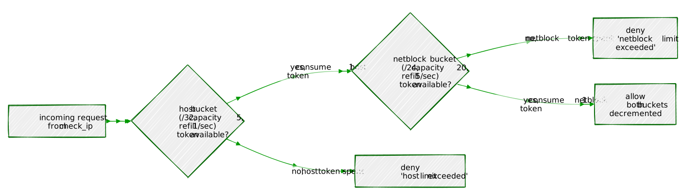
check_rate_limit(), built below, is exactly this
diagram: the host bucket is checked — and consumed — first, and only a
request that clears it goes on to spend a netblock token too.
7.3 — Schema: bucket keyed by ip4r, not
ip4
CREATE TABLE rate_limit_buckets (
bucket ip4r PRIMARY KEY,
capacity NUMERIC NOT NULL,
refill_rate NUMERIC NOT NULL,
tokens NUMERIC NOT NULL,
updated_at TIMESTAMPTZ NOT NULL DEFAULT clock_timestamp()
);Using ip4r as the key, rather than ip4 plus
a separate “is this a host or a netblock” flag, means a host bucket and
a netblock bucket are just two different-sized ranges sharing one table
and one lookup path — a host is stored as its /32, a
netblock as its /24.
7.4 — The atomic refill-and-consume function
The refill math and the allow/deny decision have to happen as one
atomic operation — two concurrent requests against the same bucket must
not both read “4 tokens available” and both proceed, the same race
Chapter 3 built FOR UPDATE SKIP LOCKED to avoid in the job
queue. Here the fix is simpler — plain FOR UPDATE, no
SKIP LOCKED — because a rate limit should make the
second concurrent request wait its turn for the lock rather than skip
ahead to a different row; there’s only one row per bucket, not a queue
of interchangeable ones:
CREATE OR REPLACE FUNCTION try_consume_bucket(
target_bucket ip4r,
p_capacity NUMERIC,
p_refill_rate NUMERIC
) RETURNS TABLE (allowed BOOLEAN, tokens_remaining NUMERIC) AS $$
BEGIN
INSERT INTO rate_limit_buckets (bucket, capacity, refill_rate, tokens, updated_at)
VALUES (target_bucket, p_capacity, p_refill_rate, p_capacity, clock_timestamp())
ON CONFLICT (bucket) DO NOTHING;
RETURN QUERY
WITH refilled AS (
SELECT b.bucket,
LEAST(b.capacity, b.tokens + b.refill_rate *
EXTRACT(EPOCH FROM (clock_timestamp() - b.updated_at))) AS available
FROM rate_limit_buckets b
WHERE b.bucket = target_bucket
FOR UPDATE
)
UPDATE rate_limit_buckets u
SET tokens = CASE WHEN r.available >= 1 THEN r.available - 1 ELSE r.available END,
updated_at = clock_timestamp()
FROM refilled r
WHERE u.bucket = r.bucket
RETURNING (r.available >= 1), u.tokens;
END;
$$ LANGUAGE plpgsql;The INSERT ... ON CONFLICT DO NOTHING lazily creates a
bucket at full capacity the first time an address is ever seen — no
separate provisioning step. Note clock_timestamp(), not
now(): this is the same gotcha from Chapter 3 —
now() freezes at transaction start, which would make every
refill calculation inside one transaction compute against the same
frozen instant instead of real elapsed wall-clock time.
7.5 — Combine host and netblock into one check
CREATE OR REPLACE FUNCTION check_rate_limit(check_ip ip4)
RETURNS TABLE (allowed BOOLEAN, reason TEXT, host_tokens NUMERIC, netblock_tokens NUMERIC) AS $$
DECLARE
host_result RECORD;
netblock_result RECORD;
BEGIN
-- Host bucket: tight limit, catches a single misbehaving address.
SELECT * INTO host_result
FROM try_consume_bucket(check_ip::ip4r, 5, 1);
IF NOT host_result.allowed THEN
RETURN QUERY SELECT FALSE, 'host limit exceeded'::TEXT, host_result.tokens_remaining, NULL::NUMERIC;
RETURN;
END IF;
-- Netblock bucket: looser limit, catches abuse spread across many
-- hosts in the same /24, each individually within their own budget.
SELECT * INTO netblock_result
FROM try_consume_bucket(ip4r_net_prefix(check_ip, 24), 20, 5);
IF NOT netblock_result.allowed THEN
RETURN QUERY SELECT FALSE, 'netblock limit exceeded'::TEXT, host_result.tokens_remaining, netblock_result.tokens_remaining;
RETURN;
END IF;
RETURN QUERY SELECT TRUE, 'ok'::TEXT, host_result.tokens_remaining, netblock_result.tokens_remaining;
END;
$$ LANGUAGE plpgsql;The host bucket (capacity 5, refills 1/sec) is checked — and, critically, consumed — first. Only if the host bucket allows the request does the function go on to check the netblock bucket (capacity 20, refills 5/sec). This ordering is a real design decision, not an accident: it means a request that the netblock bucket ultimately rejects still spent a host token on the way there. The alternative — check both before consuming either — avoids that, at the cost of two extra reads per request. For a security throttle, spending a token on a request you were going to reject anyway is a rounding error; use whichever trade-off matches what you’re actually optimizing for.
7.6 — A single host bursting past its own limit
SELECT allowed, reason, round(host_tokens, 2), round(netblock_tokens, 2)
FROM check_rate_limit('203.0.113.5');
-- run six times in a row allowed | reason | host_tokens | netblock_tokens
---------+----------------------+-------------+------------------
t | ok | 4.00 | 19.00
t | ok | 3.05 | 18.27
t | ok | 2.09 | 17.45
t | ok | 1.13 | 16.63
t | ok | 0.17 | 15.83
f | host limit exceeded | 0.20 |Five rapid calls spend the host bucket’s burst capacity of 5 (with a sliver of refill accumulating between each real request — these were genuinely separate round trips, not a batch); the sixth is denied, purely on the host bucket. The netblock bucket barely moved. (Your own numbers will differ in the small decimals — they depend on the exact wall-clock gap between your requests — but the allow/allow/allow/allow/allow/deny pattern will not.)
7.7 — Distributed abuse across a /24: the case
this whole exercise exists for
Five different hosts in the same netblock, each making five rapid requests — each individually within its own host budget:
-- for host in 203.0.113.10 .. 203.0.113.14, 5 calls each:
SELECT allowed, reason, round(host_tokens, 2), round(netblock_tokens, 2)
FROM check_rate_limit(:host); host | allowed | reason | host_tokens | netblock_tokens
-----------------+---------+--------------------------+-------------+------------------
203.0.113.10 | t | ok | 4.00 | 19.00
203.0.113.10 | t | ok | 3.04 | 18.19
203.0.113.10 | t | ok | 2.08 | 17.38
203.0.113.10 | t | ok | 1.11 | 16.57
203.0.113.10 | t | ok | 0.15 | 15.76
203.0.113.11 | t | ok | 4.00 | 14.94
203.0.113.11 | t | ok | 3.04 | 14.13
203.0.113.11 | t | ok | 2.07 | 13.32
203.0.113.11 | t | ok | 1.11 | 12.51
203.0.113.11 | t | ok | 0.15 | 11.70
203.0.113.12 | t | ok | 4.00 | 10.88
203.0.113.12 | t | ok | 3.04 | 10.07
203.0.113.12 | t | ok | 2.08 | 9.27
203.0.113.12 | t | ok | 1.11 | 8.46
203.0.113.12 | t | ok | 0.15 | 7.64
203.0.113.13 | t | ok | 4.00 | 6.82
203.0.113.13 | t | ok | 3.04 | 6.03
203.0.113.13 | t | ok | 2.08 | 5.23
203.0.113.13 | t | ok | 1.12 | 4.42
203.0.113.13 | t | ok | 0.16 | 3.62
203.0.113.14 | t | ok | 4.00 | 2.81
203.0.113.14 | t | ok | 3.04 | 2.02
203.0.113.14 | t | ok | 2.08 | 1.20
203.0.113.14 | t | ok | 1.11 | 0.38
203.0.113.14 | f | netblock limit exceeded | 0.15 | 0.56Read the host_tokens column top to bottom: every
single request succeeds at the host level — no address ever
exhausts its own bucket, each one’s burst-of-5 fits comfortably within
its own limit every time. And yet the 25th request, from the fifth host,
is denied — for netblock limit exceeded, not a host limit.
Twenty-five individually reasonable requests from five individually
well-behaved addresses added up to more than the /24 as a
whole was ever budgeted for, and the second bucket caught it. This is
precisely the pattern a per-host-only rate limiter is structurally blind
to.
| Tool | What it does |
|---|---|
ip4 / ip4r |
Dedicated address and range types — 4 and 8 bytes, versus 10 for
inet/cidr |
ip6 / ip6r / ipaddress /
iprange |
The same machinery for IPv6, and family-agnostic polymorphic types |
cidr |
Stricter than inet — rejects any value with host bits
set past the mask |
'a-b'::ip4r |
An arbitrary range, not required to be CIDR-aligned — something
cidr cannot express at all |
a >> b / b <<= a |
Containment, read from either direction — “does a
contain b?” / “is b contained by
a?” |
a && b |
Overlap — true if two ranges share any address, regardless of which contains which |
GIST (col) on ip4r |
Fast containment/overlap lookups — but only for ip4r,
ip4 has no GiST opclass |
GIST ((col::ip4r)) on ip4 |
The expression-index fix when your column stores points, not ranges |
ip4r_net_prefix(ip, n) |
Native way to compute the containing /n network for an address |
network(set_masklen(col::cidr, n)) |
The same computation via built-in
inet/cidr functions |
Token bucket, keyed by ip4r |
Rate limiting at both host (/32) and netblock
(/24) scope from one table, catching distributed abuse a
per-host limit alone can’t see |
The key design insight from this chapter is that a
blocklist and an allowlist are not just two tables you check in some
order — they are two sources of truth that will disagree, and
Exercise 5 found a real disagreement in four hand-written rows almost by
accident. A security system that doesn’t actively check for that
disagreement is trusting whichever list happens to get consulted first,
silently. && makes finding every such conflict a
single query; is_blocked() makes resolving it a permanent,
enforced policy instead of a hope.
Going further: this chapter’s is_blocked() resolves
conflicts with a fixed rule — allowlist always wins. A more nuanced
system might weight by range specificity (Exercise 4’s observation that
narrower ranges tend to be higher-confidence) or by how recently an
entry was added. For very large blocklists — commercial
threat-intelligence feeds run to millions of entries — also benchmark
GiST against ip4r’s B-tree and hash opclasses for the
access patterns that are pure equality or pure sorting rather than
containment, since GiST is the right tool specifically for range
queries, not a strictly faster B-tree replacement. And if this system
needs to block traffic in real time rather than just log a verdict, the
natural next step is exposing is_blocked() at the
application’s edge — a reverse proxy or API gateway calling it per
request — which is exactly the kind of function Chapter 10’s PostgREST
chapter would expose as an RPC endpoint. The same is true of
check_rate_limit() from Exercise 7 — a real deployment
calls it once per incoming request, before any other work happens, and a
single rate_limit_buckets table means every application
server sees the same limits regardless of which one handled the last
request, something an in-process rate limiter can’t offer without a
shared store of its own. If per-request PL/pgSQL round trips ever become
the bottleneck rather than the safeguard, that’s the point at which a
dedicated in-memory limiter (Redis and similar) starts to earn its keep
— but plenty of systems never reach the traffic level where that
trade-off is worth the added moving part.
“A table doesn’t get slow because it’s big. It gets slow because every query has to consider all of it — partitioning doesn’t shrink the table, it shrinks the part any single query has to look at.”
Every chapter so far has reached for an extension —
pg_trgm, pgvector, ip4r — to get
a data type or index PostgreSQL doesn’t ship with. This chapter is
different: declarative partitioning (since PostgreSQL 10) and BRIN
indexes (since PostgreSQL 9.5) are both built-in core features. No
CREATE EXTENSION anywhere in this chapter. What they solve
isn’t “how do I store this,” it’s “how do I keep a table that never
stops growing from turning every query, every index, and every
maintenance operation into a scan of everything that has ever
happened.”
Partitioning splits one logical table into many
physical ones, each holding a slice of the rows — by date range, by
category, by hash — while every query still just says
SELECT ... FROM sensor_readings. The planner decides,
before it reads a single row, which physical partitions could possibly
contain a match and skips the rest entirely. That’s partition
pruning, and it’s the entire value proposition: a query asking
for one month of data out of a year doesn’t pay for the other eleven
months, not even to rule them out.
BRIN (Block Range INdex) is a different kind of index for a specific shape of data: values that are large in volume but naturally correlated with physical storage order. A B-tree index stores an entry for every single row and costs roughly proportional to the row count. A BRIN index stores one small summary — just a min and max — per range of physical disk pages (128 pages by default), and costs almost nothing regardless of how many rows are in the table. The catch, and it’s a real one: BRIN only helps if physical order and value order actually correlate. For a table where rows are inserted in timestamp order and essentially never updated — exactly what an append-only sensor log looks like — the correlation is close to perfect, and that’s the case this chapter builds.
Portsmith has quietly wired up 120 sensors across the city — temperature sensors, traffic counters, and air quality monitors — all reporting on a schedule, all day, every day. A year of this is over ten million rows, and it only grows. The data starts life the way most time-series data actually starts: as one plain, unpartitioned table, because nobody provisions a partitioning scheme before they have a problem. This chapter is that problem arriving, and fixing it.
| Table | Purpose |
|---|---|
sensors |
Metadata for all 120 sensors — type, label, neighborhood/street |
sensor_readings_staging |
~10.5 million raw readings for 2024, as one unpartitioned table |
sensor_readings |
(built in this chapter) the same data, partitioned by month |
sensor_readings_by_type |
(built in this chapter) a second copy, partitioned by type and month |
sensor_readings_staging is the state the data starts in.
Building sensor_readings from it — deciding the scheme,
creating the partitions, backfilling — is the exercise, not something
handed to you already done.
By the end of this chapter you will be able to:
EXPLAIN plan well enough to tell the difference
between a query that touches one partition and one that touches all of
them.DROP TABLE on
a partition, and see exactly what that avoids compared to
DELETE on an unpartitioned table.LIST over
RANGE — into one table, and confirm the planner prunes on
both dimensions at once.Nothing to install. PARTITION BY and
USING BRIN are both part of core PostgreSQL — if
psql --version says 10 or later for partitioning, or 9.5 or
later for BRIN, you already have everything this chapter uses. (The
Portsmith cluster is PostgreSQL 16, well past both.)
python data/ch08_seed.pyExpected output (the exact seconds will vary with your machine; the row counts will not):
Connecting to: dbname=portsmith
Creating schema …
Inserting 120 sensors …
Generating and loading readings (this takes a few minutes) …
generated January 2024 — 892,800 rows
generated February 2024 — 835,200 rows
generated March 2024 — 892,800 rows
generated April 2024 — 864,000 rows
generated May 2024 — 892,800 rows
generated June 2024 — 864,000 rows
generated July 2024 — 892,800 rows
generated August 2024 — 892,800 rows
generated September 2024 — 864,000 rows
generated October 2024 — 892,800 rows
generated November 2024 — 864,000 rows
generated December 2024 — 892,800 rows
Indexing staging table on recorded_at (mirrors a typical pre-partitioning table) …
Done — 10,540,800 rows in sensor_readings_staging (131.3s to generate + load), 120 sensors.Months vary in row count because February is shorter and because temperature/traffic sensors report every 5 minutes while air quality sensors report every 15 — not a bug, just three sensor types on three different schedules, same as a real deployment would have.
SET timezone = 'UTC';This matters more than it looks like it should.
TIMESTAMPTZ values are stored as absolute instants, but a
bound like '2024-01-01' in a
CREATE TABLE ... PARTITION OF ... FOR VALUES FROM (...)
clause gets interpreted relative to the session’s timezone at the
moment the partition is created. Two people creating “the same”
January partition in two different session timezones will get two
different absolute boundaries. Run every example in this chapter in a
UTC session — this SET at the top of each psql
session is enough — and the partition boundaries and the displayed
timestamps will both match what’s printed below exactly.
Check 1 — the metadata table:
\d sensors Table "public.sensors"
Column | Type | Collation | Nullable | Default
--------------+---------+-----------+----------+---------
id | integer | | not null |
sensor_type | text | | not null |
label | text | | not null |
neighborhood | text | | not null |
Indexes:
"sensors_pkey" PRIMARY KEY, btree (id)
Check constraints:
"sensors_sensor_type_check" CHECK (sensor_type = ANY (ARRAY['temperature'::text, 'traffic'::text, 'air_quality'::text]))
Referenced by:
TABLE "sensor_readings_staging" CONSTRAINT "sensor_readings_staging_sensor_id_fkey" FOREIGN KEY (sensor_id) REFERENCES sensors(id)Check 2 — the staging table structure:
\d sensor_readings_staging Table "public.sensor_readings_staging"
Column | Type | Collation | Nullable | Default
---------------+--------------------------+-----------+----------+------------------------------
id | bigint | | not null | generated always as identity
sensor_id | integer | | not null |
sensor_type | text | | not null |
reading_value | double precision | | not null |
recorded_at | timestamp with time zone | | not null |
Indexes:
"idx_sensor_readings_staging_recorded_at" btree (recorded_at)
Check constraints:
"sensor_readings_staging_sensor_type_check" CHECK (sensor_type = ANY (ARRAY['temperature'::text, 'traffic'::text, 'air_quality'::text]))
Foreign-key constraints:
"sensor_readings_staging_sensor_id_fkey" FOREIGN KEY (sensor_id) REFERENCES sensors(id)Note this table already has a B-tree index on
recorded_at — a perfectly ordinary choice for “the column I
filter on,” and exactly what a lot of real unpartitioned time-series
tables look like right up until someone asks why disk usage keeps
climbing.
Check 3 — sensor and reading counts by type:
SELECT sensor_type, COUNT(*) FROM sensors GROUP BY sensor_type ORDER BY sensor_type; sensor_type | count
-------------+-------
air_quality | 30
temperature | 50
traffic | 40
(3 rows)SELECT sensor_type, COUNT(*) FROM sensor_readings_staging GROUP BY sensor_type ORDER BY sensor_type; sensor_type | count
-------------+---------
air_quality | 1054080
temperature | 5270400
traffic | 4216320
(3 rows)If these match, proceed to the exercises.
1.1 — Choose the partition key up front
Partitioning isn’t something you bolt onto an existing table —
PARTITION BY is part of CREATE TABLE and can’t
be added with ALTER TABLE afterward. That means the
decision has to be made before a single row is loaded into the
partitioned structure, based on how the table will actually be queried.
sensor_readings is queried almost exclusively by time range
(“show me last week,” “roll up by month”), so
RANGE (recorded_at), monthly, is the natural key — coarse
enough to keep the partition count manageable, fine enough that most
queries touch only one or two partitions.
1.2 — Create the partitioned table and its monthly partitions
CREATE TABLE sensor_readings (
id BIGINT GENERATED ALWAYS AS IDENTITY,
sensor_id INTEGER NOT NULL REFERENCES sensors(id),
sensor_type TEXT NOT NULL
CHECK (sensor_type IN ('temperature', 'traffic', 'air_quality')),
reading_value DOUBLE PRECISION NOT NULL,
recorded_at TIMESTAMPTZ NOT NULL
) PARTITION BY RANGE (recorded_at);
CREATE TABLE sensor_readings_2024_01 PARTITION OF sensor_readings FOR VALUES FROM ('2024-01-01') TO ('2024-02-01');
CREATE TABLE sensor_readings_2024_02 PARTITION OF sensor_readings FOR VALUES FROM ('2024-02-01') TO ('2024-03-01');
CREATE TABLE sensor_readings_2024_03 PARTITION OF sensor_readings FOR VALUES FROM ('2024-03-01') TO ('2024-04-01');
CREATE TABLE sensor_readings_2024_04 PARTITION OF sensor_readings FOR VALUES FROM ('2024-04-01') TO ('2024-05-01');
CREATE TABLE sensor_readings_2024_05 PARTITION OF sensor_readings FOR VALUES FROM ('2024-05-01') TO ('2024-06-01');
CREATE TABLE sensor_readings_2024_06 PARTITION OF sensor_readings FOR VALUES FROM ('2024-06-01') TO ('2024-07-01');
CREATE TABLE sensor_readings_2024_07 PARTITION OF sensor_readings FOR VALUES FROM ('2024-07-01') TO ('2024-08-01');
CREATE TABLE sensor_readings_2024_08 PARTITION OF sensor_readings FOR VALUES FROM ('2024-08-01') TO ('2024-09-01');
CREATE TABLE sensor_readings_2024_09 PARTITION OF sensor_readings FOR VALUES FROM ('2024-09-01') TO ('2024-10-01');
CREATE TABLE sensor_readings_2024_10 PARTITION OF sensor_readings FOR VALUES FROM ('2024-10-01') TO ('2024-11-01');
CREATE TABLE sensor_readings_2024_11 PARTITION OF sensor_readings FOR VALUES FROM ('2024-11-01') TO ('2024-12-01');
CREATE TABLE sensor_readings_2024_12 PARTITION OF sensor_readings FOR VALUES FROM ('2024-12-01') TO ('2025-01-01');
CREATE TABLE sensor_readings_default PARTITION OF sensor_readings DEFAULT;Each FOR VALUES FROM (...) TO (...) is a half-open
interval — inclusive of the lower bound, exclusive of the upper — so
consecutive months tile the year with no gap and no overlap. The last
one, sensor_readings_default, is not optional in any
meaningful sense: without it, any row whose recorded_at
doesn’t fall in one of the twelve defined ranges is simply rejected at
insert time. With it, such a row is accepted and routed there instead —
silently, unless you go looking. Exercise 2 finds a case where that’s
exactly what happens.
1.3 — Confirm the structure
\d sensor_readings Partitioned table "public.sensor_readings"
Column | Type | Collation | Nullable | Default
---------------+--------------------------+-----------+----------+------------------------------
id | bigint | | not null | generated always as identity
sensor_id | integer | | not null |
sensor_type | text | | not null |
reading_value | double precision | | not null |
recorded_at | timestamp with time zone | | not null |
Partition key: RANGE (recorded_at)
Check constraints:
"sensor_readings_sensor_type_check" CHECK (sensor_type = ANY (ARRAY['temperature'::text, 'traffic'::text, 'air_quality'::text]))
Foreign-key constraints:
"sensor_readings_sensor_id_fkey" FOREIGN KEY (sensor_id) REFERENCES sensors(id)
Number of partitions: 13 (Use \d+ to list them.)sensor_readings itself has no storage of its own — it’s
a routing target. Every row you insert into it physically lands in
exactly one of the thirteen tables underneath.
2.1 — Backfill from staging
INSERT INTO sensor_readings (sensor_id, sensor_type, reading_value, recorded_at)
SELECT sensor_id, sensor_type, reading_value, recorded_at
FROM sensor_readings_staging;INSERT 0 10540800
Time: 87814.162 ms (01:27.814)One INSERT ... SELECT, no destination named beyond
sensor_readings itself — PostgreSQL evaluates each row’s
recorded_at against the partition bounds and routes it to
the matching child table. Nothing in this statement says which of the
thirteen tables any given row ends up in.
2.2 — Confirm the routing, per partition
SELECT tableoid::regclass AS partition, COUNT(*)
FROM sensor_readings
GROUP BY tableoid
ORDER BY 1; partition | count
--------------------------+--------
sensor_readings_2024_01 | 892800
sensor_readings_2024_02 | 835200
sensor_readings_2024_03 | 892800
sensor_readings_2024_04 | 864000
sensor_readings_2024_05 | 892800
sensor_readings_2024_06 | 864000
sensor_readings_2024_07 | 892800
sensor_readings_2024_08 | 892800
sensor_readings_2024_09 | 864000
sensor_readings_2024_10 | 892800
sensor_readings_2024_11 | 864000
sensor_readings_2024_12 | 891648
sensor_readings_default | 1152
(13 rows)tableoid is a hidden system column every table has, and
on a partitioned table it tells you which physical partition a given row
actually lives in — the only reliable way to ask “where did this row end
up?” after the fact.
2.3 — The row count that should stop you
Every month has the row count you’d expect from Exercise 0’s per-type
counts — except December, which is short exactly 1,152 rows, and
sensor_readings_default, which has exactly 1,152 rows in
it. That’s not a coincidence:
SELECT sensor_id, MIN(recorded_at), MAX(recorded_at), COUNT(*)
FROM sensor_readings
WHERE tableoid = 'sensor_readings_default'::regclass
GROUP BY sensor_id; sensor_id | min | max | count
-----------+-------------------------+-------------------------+-------
17 | 2025-12-27 00:00:00+00 | 2025-12-31 23:55:00+00 | 1152Sensor 17 — a temperature sensor — has a clock bug: for its last four
days of reporting, it stamped its readings a full year fast. Nothing
about the INSERT failed or warned; the rows are sitting
exactly where the schema said out-of-range data should go. This is
precisely the scenario a DEFAULT partition exists for, and
precisely why “does the default partition have anything in it?” is worth
checking after any real backfill, not just this synthetic one — it’s the
difference between a sensor firmware bug you catch in five minutes and
one you catch when someone asks why a report is missing a device.
EXPLAIN3.1 — A date-filtered query touches one partition
EXPLAIN (ANALYZE, BUFFERS)
SELECT sensor_type, COUNT(*), round(AVG(reading_value)::numeric, 2)
FROM sensor_readings
WHERE recorded_at >= '2024-06-01' AND recorded_at < '2024-07-01'
GROUP BY sensor_type
ORDER BY sensor_type; Finalize GroupAggregate (cost=12411.99..12480.46 rows=200 width=72) (actual time=182.595..203.871 rows=3 loops=1)
Group Key: sensor_readings.sensor_type
Buffers: shared hit=106 read=7168, temp read=3264 written=3276
-> Gather Merge (cost=12411.99..12473.96 rows=400 width=72) (actual time=152.757..203.835 rows=9 loops=1)
Workers Planned: 2
Workers Launched: 2
-> Partial GroupAggregate (cost=11411.97..11427.77 rows=200 width=72) (actual time=98.794..149.785 rows=3 loops=3)
Group Key: sensor_readings.sensor_type
-> Sort (cost=11411.97..11415.42 rows=1380 width=40) (actual time=93.166..120.544 rows=288000 loops=3)
Sort Key: sensor_readings.sensor_type
Sort Method: external merge Disk: 8720kB
-> Parallel Seq Scan on sensor_readings_2024_06 sensor_readings (cost=0.00..11340.00 rows=1380 width=40) (actual time=0.034..37.199 rows=288000 loops=3)
Filter: ((recorded_at >= '2024-06-01 00:00:00+00'::timestamp with time zone) AND (recorded_at < '2024-07-01 00:00:00+00'::timestamp with time zone))
Planning Time: 6.417 ms
Execution Time: 205.458 msThe GROUP BY sensor_type on top adds a sort and some
parallel-worker bookkeeping that isn’t the point here — the line that
matters is Parallel Seq Scan on sensor_readings_2024_06,
singular. Eleven other monthly partitions and the default partition
exist; none of them appear anywhere in this plan. The planner threw them
out during planning, before execution ever started, based purely on the
WHERE clause matching only June’s range.
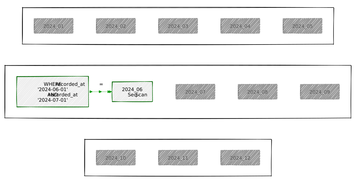
3.2 — The same query, no date filter, for contrast
EXPLAIN
SELECT sensor_type, COUNT(*)
FROM sensor_readings
GROUP BY sensor_type; Finalize GroupAggregate (cost=156197.01..156247.68 rows=200 width=40)
-> Gather Merge (cost=156197.01..156243.68 rows=400 width=40)
-> Sort (cost=155196.99..155197.49 rows=200 width=40)
-> Partial HashAggregate (cost=155187.34..155189.34 rows=200 width=40)
-> Parallel Append (cost=0.00..138351.15 rows=3367238 width=32)
-> Parallel Seq Scan on sensor_readings_2024_01 sensor_readings_1 ...
-> Parallel Seq Scan on sensor_readings_2024_03 sensor_readings_3 ...
-> Parallel Seq Scan on sensor_readings_2024_05 sensor_readings_5 ...
-> Parallel Seq Scan on sensor_readings_2024_07 sensor_readings_7 ...
-> Parallel Seq Scan on sensor_readings_2024_08 sensor_readings_8 ...
-> Parallel Seq Scan on sensor_readings_2024_10 sensor_readings_10 ...
-> Parallel Seq Scan on sensor_readings_2024_12 sensor_readings_12 ...
-> Parallel Seq Scan on sensor_readings_2024_04 sensor_readings_4 ...
-> Parallel Seq Scan on sensor_readings_2024_06 sensor_readings_6 ...
-> Parallel Seq Scan on sensor_readings_2024_09 sensor_readings_9 ...
-> Parallel Seq Scan on sensor_readings_2024_11 sensor_readings_11 ...
-> Parallel Seq Scan on sensor_readings_2024_02 sensor_readings_2 ...
-> Parallel Seq Scan on sensor_readings_default sensor_readings_13 ...With nothing to prune on, every one of the thirteen partitions shows
up as its own Parallel Seq Scan under a
Parallel Append. This is the direct, visible contrast:
pruning isn’t a performance optimization happening invisibly under the
hood, it’s a specific number of Seq Scan lines disappearing
from the plan, and you can watch it happen by adding or removing a date
filter on the exact same query.
4.1 — Why this data is a good fit for BRIN
BRIN’s usefulness rests entirely on physical/value correlation — do
rows with nearby recorded_at values actually sit near each
other on disk? Since this data was generated and loaded in chronological
order and never updated, it should be close to perfectly correlated:
ANALYZE sensor_readings;
SELECT tablename, attname, correlation, n_distinct
FROM pg_stats
WHERE tablename = 'sensor_readings_2024_09' AND attname = 'recorded_at'; tablename | attname | correlation | n_distinct
--------------------------+-------------+-------------+------------
sensor_readings_2024_09 | recorded_at | 0.99979776 | 8622correlation ranges from -1 to 1; 0.9998 is
as close to “physically sorted by this column” as real data gets. This
is the number that decides whether BRIN is a good idea here — not the
row count, not the table size.
4.2 — Build both indexes on one partition, compare cost to build and size
CREATE INDEX idx_sr_2024_09_brin ON sensor_readings_2024_09 USING BRIN (recorded_at);
CREATE INDEX idx_sr_2024_09_btree ON sensor_readings_2024_09 USING BTREE (recorded_at);CREATE INDEX
Time: 122.619 ms
CREATE INDEX
Time: 249.923 msSELECT relname, pg_size_pretty(pg_relation_size(oid)) AS index_size
FROM pg_class
WHERE relname IN ('idx_sr_2024_09_brin', 'idx_sr_2024_09_btree'); relname | index_size
-----------------------+------------
idx_sr_2024_09_brin | 24 kB
idx_sr_2024_09_btree | 5800 kB864,000 rows in this partition. The B-tree costs 5.8 MB — one entry per row, roughly what you’d expect. The BRIN index costs 24 KB: about 240 times smaller, because it isn’t storing one entry per row, it’s storing one min/max pair per 128-page block range — a few thousand summaries instead of 864,000 index entries. It also built about twice as fast. Neither number changes much if the table has a hundred million rows instead of 864,000; a B-tree’s cost scales with row count, BRIN’s scales with table pages, and pages-per-block-range is fixed.
4.3 — What that size difference costs you at query time
Force each index in turn and run the same narrow range query — one day out of the month:
SET enable_seqscan = off;
DROP INDEX idx_sr_2024_09_btree; -- isolate the BRIN index
EXPLAIN (ANALYZE, BUFFERS)
SELECT COUNT(*), round(AVG(reading_value)::numeric, 2)
FROM sensor_readings_2024_09
WHERE recorded_at >= '2024-09-15' AND recorded_at < '2024-09-16'; Aggregate (cost=7818.29..7818.30 rows=1 width=40) (actual time=7.350..7.351 rows=1 loops=1)
Buffers: shared hit=9 read=384
-> Bitmap Heap Scan on sensor_readings_2024_09 (cost=19.27..7674.10 rows=28836 width=8) (actual time=0.635..5.708 rows=28800 loops=1)
Recheck Cond: ((recorded_at >= '2024-09-15 00:00:00+00'::timestamp with time zone) AND (recorded_at < '2024-09-16 00:00:00+00'::timestamp with time zone))
Rows Removed by Index Recheck: 17280
Heap Blocks: lossy=384
Buffers: shared hit=9 read=384
-> Bitmap Index Scan on idx_sr_2024_09_brin (cost=0.00..12.06 rows=30322 width=0) (actual time=0.060..0.060 rows=3840 loops=1)
Index Cond: ((recorded_at >= '2024-09-15 00:00:00+00'::timestamp with time zone) AND (recorded_at < '2024-09-16 00:00:00+00'::timestamp with time zone))
Execution Time: 7.493 msHeap Blocks: lossy=384 and
Rows Removed by Index Recheck: 17280 are BRIN being honest
about what it is: a lossy index. It doesn’t know which
rows in a matching block range satisfy the condition, only that the
range’s min/max could contain a match — so it hands back every
block in range and PostgreSQL rechecks the actual condition row by row
once the blocks are read. That recheck cost is real, and it’s the trade
for the 240x smaller index.
Now the B-tree, same query:
DROP INDEX idx_sr_2024_09_brin;
CREATE INDEX idx_sr_2024_09_btree ON sensor_readings_2024_09 USING BTREE (recorded_at);
EXPLAIN (ANALYZE, BUFFERS)
SELECT COUNT(*), round(AVG(reading_value)::numeric, 2)
FROM sensor_readings_2024_09
WHERE recorded_at >= '2024-09-15' AND recorded_at < '2024-09-16'; Aggregate (cost=1076.88..1076.89 rows=1 width=40) (actual time=5.781..5.782 rows=1 loops=1)
Buffers: shared hit=384 read=27
-> Index Scan using idx_sr_2024_09_btree on sensor_readings_2024_09 (cost=0.42..932.69 rows=28836 width=8) (actual time=0.055..3.552 rows=28800 loops=1)
Index Cond: ((recorded_at >= '2024-09-15 00:00:00+00'::timestamp with time zone) AND (recorded_at < '2024-09-16 00:00:00+00'::timestamp with time zone))
Execution Time: 5.850 ms5.85 ms for the B-tree against 7.49 ms for BRIN — the B-tree is genuinely a bit faster here, exact and recheck-free by construction. But look at what each one costs to get that: 5.8 MB of index versus 24 KB, on one month of one partition. At the scale this chapter’s title implies — many partitions, much more than a year of data — a B-tree on every partition’s timestamp column stops being “a bit more disk” and starts being a meaningful fraction of the table’s own size, while BRIN stays essentially free. For an append-only, time-correlated column like this one, that trade is rarely close.
4.4 — Keep the BRIN index, drop the comparison B-tree
DROP INDEX idx_sr_2024_09_btree;
CREATE INDEX idx_sr_2024_09_brin ON sensor_readings_2024_09 USING BRIN (recorded_at);
RESET enable_seqscan;Recreate this same USING BRIN (recorded_at) index on
every other monthly partition before moving on — Exercise 5 will drop
one of them whole, and Exercise 6 revisits the size question at the
whole-table level.
DELETE5.1 — Time the unpartitioned way:
DELETE
sensor_readings_staging is still sitting there,
unpartitioned, exactly as it was before this chapter touched anything.
Delete a month’s worth of rows from it the only way an unpartitioned
table allows:
DELETE FROM sensor_readings_staging
WHERE recorded_at >= '2024-01-01' AND recorded_at < '2024-02-01';DELETE 892800
Time: 815.293 ms5.2 — Time the partitioned way:
DROP TABLE
DROP TABLE sensor_readings_2024_01;DROP TABLE
Time: 17.489 msSame amount of data — the January 2024 slice, 892,800 rows either way
— and dropping the partition is roughly 47 times faster
than deleting the equivalent rows. That gap isn’t a fluke of this
particular run: it’s two operations of fundamentally different cost.
DELETE is an MVCC operation — PostgreSQL has to visit every
matching row, mark each one dead, and write a WAL record for each one,
transaction-safely, one row at a time. DROP TABLE on a
partition is a catalog operation — it removes one entry saying “this
table is part of that partition set” and unlinks the file. No row is
individually touched because no row was individually anything; the whole
partition was always one physical object.
5.3 — The part DELETE doesn’t
finish
SELECT n_live_tup, n_dead_tup, pg_size_pretty(pg_relation_size('sensor_readings_staging'))
FROM pg_stat_user_tables
WHERE relname = 'sensor_readings_staging'; n_live_tup | n_dead_tup | pg_size_pretty
------------+------------+----------------
9648230 | 892800 | 687 MB892,800 dead tuples, exactly matching what was just deleted — and the
table is still 687 MB, unchanged, because DELETE doesn’t
reclaim disk space, it just marks rows as no-longer-visible. Getting
that space back needs a VACUUM (or VACUUM FULL
to actually shrink the file), which is its own I/O-heavy pass over the
table, usually running sometime later via autovacuum rather than as part
of the DELETE itself. DROP TABLE skipped all
of this — there is no bloat to vacuum, because there’s no table left to
have any.
5.4 — A gotcha worth knowing about before it surprises you
SELECT pg_size_pretty(pg_total_relation_size('sensor_readings')); pg_size_pretty
----------------
0 bytesThat’s not an error and the data is not gone —
pg_total_relation_size() on a partitioned table
reports only the parent’s own storage, and a partitioned table’s parent
has none; all the bytes live in the child partitions. To get the real
total, sum across the children:
SELECT pg_size_pretty(SUM(pg_total_relation_size(inhrelid))) AS total_size
FROM pg_inherits
WHERE inhparent = 'sensor_readings'::regclass; total_size
------------
629 MB5.5 — Clean up the staging table
It’s done its job — everything from here on works from
sensor_readings:
DROP TABLE sensor_readings_staging;LIST and RANGE:
Subpartitioning6.1 — Why one partition key isn’t always enough
sensor_readings prunes beautifully on date, but a query
that also filters on sensor_type — “just the traffic
sensors” — still has to scan a whole month’s worth of every sensor type,
because sensor_type isn’t part of the partition key at all.
PostgreSQL allows a second level: partition by
LIST (sensor_type) at the top, then partition each of
those by RANGE (recorded_at) underneath — a partition
of a partition, usually called subpartitioning. Two routing decisions,
made independently, before a row ever reaches physical storage:
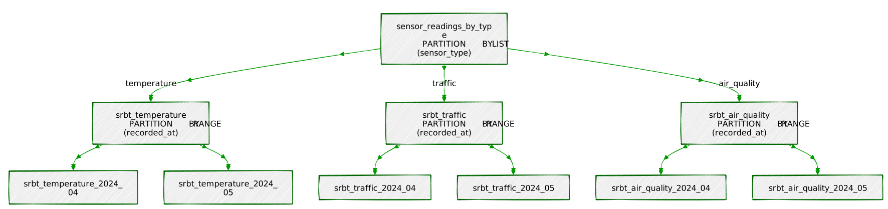
The root and the three type branches hold no data of their own — they
exist purely to route a row one level further down. Only the nine boxes
at the bottom are real tables with real storage, and every one of this
chapter’s rows lives in exactly one of them, decided first by
sensor_type, then by which month recorded_at
falls in.
6.2 — Build the two-level hierarchy
CREATE TABLE sensor_readings_by_type (
id BIGINT GENERATED ALWAYS AS IDENTITY,
sensor_id INTEGER NOT NULL,
sensor_type TEXT NOT NULL
CHECK (sensor_type IN ('temperature', 'traffic', 'air_quality')),
reading_value DOUBLE PRECISION NOT NULL,
recorded_at TIMESTAMPTZ NOT NULL
) PARTITION BY LIST (sensor_type);
CREATE TABLE srbt_temperature PARTITION OF sensor_readings_by_type
FOR VALUES IN ('temperature') PARTITION BY RANGE (recorded_at);
CREATE TABLE srbt_traffic PARTITION OF sensor_readings_by_type
FOR VALUES IN ('traffic') PARTITION BY RANGE (recorded_at);
CREATE TABLE srbt_air_quality PARTITION OF sensor_readings_by_type
FOR VALUES IN ('air_quality') PARTITION BY RANGE (recorded_at);
-- Three months of subpartitions under each type branch:
CREATE TABLE srbt_temperature_2024_04 PARTITION OF srbt_temperature FOR VALUES FROM ('2024-04-01') TO ('2024-05-01');
CREATE TABLE srbt_temperature_2024_05 PARTITION OF srbt_temperature FOR VALUES FROM ('2024-05-01') TO ('2024-06-01');
CREATE TABLE srbt_temperature_2024_06 PARTITION OF srbt_temperature FOR VALUES FROM ('2024-06-01') TO ('2024-07-01');
CREATE TABLE srbt_traffic_2024_04 PARTITION OF srbt_traffic FOR VALUES FROM ('2024-04-01') TO ('2024-05-01');
CREATE TABLE srbt_traffic_2024_05 PARTITION OF srbt_traffic FOR VALUES FROM ('2024-05-01') TO ('2024-06-01');
CREATE TABLE srbt_traffic_2024_06 PARTITION OF srbt_traffic FOR VALUES FROM ('2024-06-01') TO ('2024-07-01');
CREATE TABLE srbt_air_quality_2024_04 PARTITION OF srbt_air_quality FOR VALUES FROM ('2024-04-01') TO ('2024-05-01');
CREATE TABLE srbt_air_quality_2024_05 PARTITION OF srbt_air_quality FOR VALUES FROM ('2024-05-01') TO ('2024-06-01');
CREATE TABLE srbt_air_quality_2024_06 PARTITION OF srbt_air_quality FOR VALUES FROM ('2024-06-01') TO ('2024-07-01');Three months only, and only as a working example — building out all twelve for all three types is the same pattern repeated, not a new idea, and this chapter’s disk budget would rather spend on data than on empty demonstration partitions.
6.3 — Backfill from sensor_readings and inspect
the tree
INSERT INTO sensor_readings_by_type (sensor_id, sensor_type, reading_value, recorded_at)
SELECT sensor_id, sensor_type, reading_value, recorded_at
FROM sensor_readings
WHERE recorded_at >= '2024-04-01' AND recorded_at < '2024-07-01';INSERT 0 2620800
Time: 3389.698 ms (00:03.390)SELECT relid::regclass AS relation, parentrelid::regclass AS parent, isleaf, level
FROM pg_partition_tree('sensor_readings_by_type')
ORDER BY level, 1; relation | parent | isleaf | level
--------------------------+-------------------------+--------+-------
sensor_readings_by_type | | f | 0
srbt_air_quality | sensor_readings_by_type | f | 1
srbt_temperature | sensor_readings_by_type | f | 1
srbt_traffic | sensor_readings_by_type | f | 1
srbt_air_quality_2024_04 | srbt_air_quality | t | 2
srbt_air_quality_2024_05 | srbt_air_quality | t | 2
srbt_air_quality_2024_06 | srbt_air_quality | t | 2
srbt_temperature_2024_04 | srbt_temperature | t | 2
srbt_temperature_2024_05 | srbt_temperature | t | 2
srbt_temperature_2024_06 | srbt_temperature | t | 2
srbt_traffic_2024_04 | srbt_traffic | t | 2
srbt_traffic_2024_05 | srbt_traffic | t | 2
srbt_traffic_2024_06 | srbt_traffic | t | 2
(13 rows)pg_partition_tree() is the built-in way to see this
shape directly instead of inferring it from table names: one root, three
LIST branches at level 1, nine RANGE leaves at
level 2 — every row actually lives in one of those nine leaf tables,
never in an intermediate one.
6.4 — Confirm pruning happens on both dimensions at once
EXPLAIN (ANALYZE, BUFFERS)
SELECT COUNT(*), round(AVG(reading_value)::numeric, 2)
FROM sensor_readings_by_type
WHERE sensor_type = 'traffic'
AND recorded_at >= '2024-05-01' AND recorded_at < '2024-06-01'; Finalize Aggregate (cost=6794.58..6794.60 rows=1 width=40) (actual time=37.692..40.669 rows=1 loops=1)
-> Gather (cost=6794.47..6794.58 rows=1 width=40) (actual time=37.612..40.655 rows=2 loops=1)
Workers Planned: 1
-> Partial Aggregate (cost=5794.47..5794.48 rows=1 width=40) (actual time=36.350..36.351 rows=1 loops=2)
-> Parallel Seq Scan on srbt_traffic_2024_05 sensor_readings_by_type (cost=0.00..5794.45 rows=4 width=8) (actual time=0.018..26.204 rows=178560 loops=2)
Filter: ((recorded_at >= '2024-05-01 00:00:00+00'::timestamp with time zone) AND (recorded_at < '2024-06-01 00:00:00+00'::timestamp with time zone) AND (sensor_type = 'traffic'::text))
Execution Time: 40.738 msOne line, Parallel Seq Scan on srbt_traffic_2024_05, out
of the nine leaf partitions that exist. The
sensor_type = 'traffic' predicate pruned two of the three
top-level branches before the range predicate even got involved, and the
range predicate then pruned two of that branch’s three months. Both
partition keys did real work on this single query, independently, in the
same plan.
| Tool | What it does |
|---|---|
PARTITION BY RANGE (col) |
Split a table into physical children by value range on one column — the whole table stays queryable as one name |
FOR VALUES FROM (...) TO (...) |
Half-open interval defining one range partition’s bounds |
... DEFAULT partition |
Catches any row that doesn’t match a defined range — without one, out-of-range inserts are rejected outright |
tableoid::regclass |
Ask which physical partition a given row actually lives in |
| Partition pruning | The planner drops non-matching partitions from the plan
before execution, visible as missing Seq Scan
lines in EXPLAIN |
USING BRIN (col) |
Index storing one min/max summary per block range — tiny and cheap, but only useful when physical and value order correlate |
correlation in pg_stats |
The number that tells you whether BRIN is actually a good idea for a given column |
DROP TABLE on a partition |
Metadata-only, near-instant removal of a whole partition’s worth of data — no per-row MVCC cost, no bloat to vacuum afterward |
pg_total_relation_size() on a partitioned table |
Reports the (empty) parent only — sum over pg_inherits
for the real total |
PARTITION BY LIST over
PARTITION BY RANGE |
Subpartitioning — two partition keys, pruned independently, in one query plan |
pg_partition_tree() |
Walk a partition hierarchy — root, branches, and leaves — as a query instead of by table-naming convention |
The key design insight from this chapter is that partitioning and indexing solve different halves of the same problem, and BRIN sits exactly at their intersection. Partition pruning throws away whole partitions the planner can prove are irrelevant, cutting the search space by orders of magnitude before a single row is touched. BRIN then indexes what’s left almost for free, precisely because append-only, time-ordered data — the same shape of data that makes range partitioning by date the obvious choice — is also the shape that makes a physically-correlated, lossy index a good trade instead of a bad one. Neither technique is really “for time-series data” in the abstract; both are for data whose physical order already tells you something true about its values, and this chapter’s sensor readings happen to be exactly that.
Going further: hand-writing twelve
CREATE TABLE ... PARTITION OF statements a year, forever,
is exactly the kind of recurring maintenance that Chapter 19’s
pg_cron is suited to automate — schedule a monthly job that
creates next month’s partition before it’s needed and, if a retention
policy allows it, drops the oldest one the same way Exercise 5 did by
hand. In production this whole lifecycle — creation, retention, even the
migration of aging partitions to cheaper storage — is usually handled by
the pg_partman extension rather than bespoke scripts;
everything in this chapter is what pg_partman is automating
under the hood, which is worth knowing before reaching for it, not
instead of. sensor_readings also isn’t done being useful:
Chapter 9’s materialized views roll it up into daily summaries without
re-scanning raw readings each time, Chapter 11’s window functions
compute rolling averages and day-over-day deltas across it, and Chapter
16 adds a generated reading_date column to make date-only
grouping cheaper still. And a caution in the other direction — BRIN is
not a free upgrade for every index. A column with low correlation (a
randomly- assigned sensor_id, say, rather than an
ever-increasing timestamp) gets none of BRIN’s benefit and most of a
sequential scan’s cost, because every block range ends up spanning the
entire value domain. Check correlation before reaching for
BRIN, the same way Exercise 4 did here — it’s a bet on the physical
shape of your data, not a strictly smaller B-tree.
“A view is a promise to run the query again. A materialized view is a promise it already kept — until you ask it to keep it again.”
A plain VIEW is a saved query, nothing more. Every time
you SELECT from one, PostgreSQL substitutes the view’s
definition in place and runs the underlying query from scratch. That’s
fine for a view whose job is convenience — hiding a join, naming a
filter — but it’s a bad deal for a view whose job is a genuinely
expensive aggregation. If a dashboard asks “average sensor reading per
day, per type, for the whole year” a hundred times a day, a plain view
answers that question by scanning millions of raw rows a hundred times a
day, even though the answer barely changes between asks.
A MATERIALIZED VIEW is the other end of that trade: it
runs the query once, writes the result to disk as an honest-to-goodness
physical table, and answers every subsequent SELECT from
that table instead of the original data. It can be indexed like any
table, because it is a table underneath a SELECT
definition it remembers. The cost moves from “every read pays the full
aggregation” to “one write pays the full aggregation, and reads are
cheap until you explicitly ask for a refresh.” Nothing about it is
automatic — that’s the whole trade. A materialized view does not notice
that its source data changed. It sits there, confidently wrong, until
something runs REFRESH MATERIALIZED VIEW.
That puts a materialized view in between two other tools you already have. A plain view is always correct and never fast. A hand-maintained summary table — one your application code writes to directly, in the same transaction as the data that feeds it — can be both correct and fast, but you own every line of the code that keeps it that way. A materialized view sits in the middle: PostgreSQL owns the how (it already knows how to run the query), you own the when (deciding on a refresh policy is the actual engineering decision this chapter is about).

Portsmith’s ops team wants a dashboard: daily and monthly rollups of
the sensor network from Chapter 8 — average readings, counts, mins and
maxes, sliced by day and sensor type. sensor_readings now
holds 9,648,000 rows across eleven monthly partitions plus a default
partition, and it only grows. Nobody wants the dashboard to re-scan that
on every page load, and nobody wants to hand-write application code that
keeps a summary table in sync by hand either. This chapter builds the
rollups as materialized views instead, and spends its exercises on the
part that’s actually hard about them: deciding how and when they get
refreshed.
| Object | Purpose |
|---|---|
sensor_readings |
(from Chapter 8) 9,648,000 partitioned sensor readings, Feb–Dec 2024 |
mv_sensor_daily |
(built in this chapter) one row per day per sensor type |
mv_sensor_monthly |
(built in this chapter) mv_sensor_daily rolled
up one level further |
matview_refresh_log |
(built in this chapter) tracks when each matview was last refreshed |
By the end of this chapter you will be able to:
WITH DATA
vs. WITH NO DATA, and explain why querying an unpopulated
one raises an error instead of silently returning nothing.EXPLAIN ANALYZE numbers, exactly
what a materialized view saves compared to the raw aggregate it
replaces.REFRESH MATERIALIZED VIEW CONCURRENTLY requires, and prove
— with two open sessions — what it actually buys you over a plain
REFRESH.pg_cron.pg_matviews, PostgreSQL’s own catalog for the object, has
no column that tells you when one was last refreshed.Nothing to install. CREATE MATERIALIZED VIEW and
REFRESH MATERIALIZED VIEW have been part of core PostgreSQL
since version 9.3. This chapter uses no extensions.
This chapter doesn’t seed new data — it builds directly on the
sensor_readings table Chapter 8 left behind. That matters
for two specific reasons, both consequences of exercises Chapter 8
already ran:
sensor_readings_2024_01 on purpose, to demonstrate instant
partition drop. sensor_readings now covers February through
December 2024 only.sensor_readings_default. Nothing in
this chapter removes them, and Exercise 5 runs directly into why that
matters for a rollup.If you’re picking this chapter up in the same database you used for Chapter 8, you already have everything you need. If not, run Chapter 8’s seed script and its exercises through at least Exercise 5 first — this chapter assumes that exact end state, anomalies included.
SET timezone = 'UTC';Same reason as Chapter 8: date boundaries in this chapter’s
GROUP BY clauses are computed with date_trunc,
which resolves relative to the session timezone. Run every example here
in a UTC session.
SELECT tableoid::regclass AS partition, COUNT(*)
FROM sensor_readings
GROUP BY tableoid
ORDER BY 1; partition | count
--------------------------+---------
sensor_readings_2024_02 | 835200
sensor_readings_2024_03 | 892800
sensor_readings_2024_04 | 864000
sensor_readings_2024_05 | 892800
sensor_readings_2024_06 | 864000
sensor_readings_2024_07 | 892800
sensor_readings_2024_08 | 892800
sensor_readings_2024_09 | 864000
sensor_readings_2024_10 | 892800
sensor_readings_2024_11 | 864000
sensor_readings_2024_12 | 891648
sensor_readings_default | 1152
(12 rows)Twelve partitions (no January), summing to 9,648,000 rows. If your counts match, proceed.
1.1 — Build the materialized view
CREATE MATERIALIZED VIEW mv_sensor_daily AS
SELECT
date_trunc('day', recorded_at)::date AS reading_day,
sensor_type,
COUNT(*) AS reading_count,
round(AVG(reading_value)::numeric, 2) AS avg_value,
round(MIN(reading_value)::numeric, 2) AS min_value,
round(MAX(reading_value)::numeric, 2) AS max_value
FROM sensor_readings
GROUP BY 1, 2
WITH DATA;SELECT 1010
Time: 6821.437 ms (00:06.821)Syntactically this is CREATE TABLE AS with a memory: the
SELECT that built it is stored alongside the data, which is
what makes REFRESH possible later. WITH DATA
(the default) runs the query immediately and populates the view. 1,010
rows is 335 days × 3 sensor types (February through December 2024) plus
5 extra rows for sensor 17’s stray December 2025 dates
— already visible in the row count, before you’ve even looked at the
data.
1.2 — WITH NO DATA, and the error it sets
up
CREATE MATERIALIZED VIEW mv_sensor_daily_empty AS
SELECT date_trunc('day', recorded_at)::date AS reading_day, sensor_type, COUNT(*)
FROM sensor_readings
GROUP BY 1, 2
WITH NO DATA;
SELECT * FROM mv_sensor_daily_empty LIMIT 1;CREATE MATERIALIZED VIEW
Time: 8.213 ms
ERROR: materialized view "mv_sensor_daily_empty" has not been populated
HINT: Use the REFRESH MATERIALIZED VIEW command.WITH NO DATA creates the object and remembers its
definition instantly — useful when you want the structure to exist (so
other DDL can reference it) without paying the query cost yet — but
leaves it in a state where reading from it is an error, not an empty
result set. pg_matviews.ispopulated tracks exactly
this:
SELECT matviewname, ispopulated FROM pg_matviews ORDER BY matviewname; matviewname | ispopulated
-------------------------+-------------
mv_sensor_daily | t
mv_sensor_daily_empty | f
(2 rows)DROP MATERIALIZED VIEW mv_sensor_daily_empty;That was only to show the error — it isn’t needed going forward.
1.3 — Confirm it’s a real table
SELECT pg_size_pretty(pg_total_relation_size('mv_sensor_daily')); pg_size_pretty
----------------
96 kB1,010 rows of six columns, versus 9.6 million raw rows the query underneath it scanned to produce them. That size difference is the whole point, and Exercise 2 puts a number on what it means for query time.
2.1 — Time the raw aggregate
EXPLAIN (ANALYZE, BUFFERS)
SELECT date_trunc('day', recorded_at)::date AS reading_day,
sensor_type,
COUNT(*) AS reading_count,
round(AVG(reading_value)::numeric, 2) AS avg_value
FROM sensor_readings
GROUP BY 1, 2; Finalize HashAggregate (cost=201448.99..201459.09 rows=1010 width=44) (actual time=693.128..701.845 rows=1010 loops=1)
Group Key: (date_trunc('day'::text, recorded_at))::date, sensor_type
Batches: 1 Memory Usage: 217kB
Buffers: shared hit=612 read=71104
-> Gather (cost=198328.11..201418.99 rows=3030 width=44) (actual time=210.442..688.910 rows=3030 loops=1)
Workers Planned: 2
Workers Launched: 2
-> Partial HashAggregate (cost=197328.11..197359.21 rows=1010 width=44) (actual time=195.223..637.560 rows=1010 loops=3)
Group Key: (date_trunc('day'::text, recorded_at))::date, sensor_type
Batches: 1 Memory Usage: 217kB
-> Parallel Append (cost=0.00..185004.00 rows=4022667 width=16) (actual time=0.028..312.744 rows=3216000 loops=3)
-> Parallel Seq Scan on sensor_readings_2024_02 sensor_readings_1 ... (actual time=0.031..24.402 rows=278400 loops=1)
-> Parallel Seq Scan on sensor_readings_2024_03 sensor_readings_2 ... (actual time=0.019..25.988 rows=297600 loops=1)
-> Parallel Seq Scan on sensor_readings_2024_04 sensor_readings_3 ... (actual time=0.022..24.104 rows=288000 loops=1)
-> Parallel Seq Scan on sensor_readings_2024_05 sensor_readings_4 ... (actual time=0.020..25.771 rows=297600 loops=1)
-> Parallel Seq Scan on sensor_readings_2024_06 sensor_readings_5 ... (actual time=0.021..23.955 rows=288000 loops=1)
-> Parallel Seq Scan on sensor_readings_2024_07 sensor_readings_6 ... (actual time=0.018..25.812 rows=297600 loops=1)
-> Parallel Seq Scan on sensor_readings_2024_08 sensor_readings_7 ... (actual time=0.024..25.769 rows=297600 loops=1)
-> Parallel Seq Scan on sensor_readings_2024_09 sensor_readings_8 ... (actual time=0.017..23.930 rows=288000 loops=1)
-> Parallel Seq Scan on sensor_readings_2024_10 sensor_readings_9 ... (actual time=0.021..25.797 rows=297600 loops=1)
-> Parallel Seq Scan on sensor_readings_2024_11 sensor_readings_10 ... (actual time=0.019..23.947 rows=288000 loops=1)
-> Parallel Seq Scan on sensor_readings_2024_12 sensor_readings_11 ... (actual time=0.023..25.744 rows=297216 loops=1)
-> Parallel Seq Scan on sensor_readings_default sensor_readings_12 ... (actual time=0.008..0.301 rows=384 loops=1)
Planning Time: 3.912 ms
Execution Time: 703.187 msEvery partition shows up — this query has no WHERE
clause, so nothing gets pruned, exactly as Chapter 8, Exercise 3.2
predicted. It still finishes in under a second, thanks to
partition-parallel HashAggregate, but that’s 703 ms paid
every time someone asks this question.
2.2 — Time the same question against the matview
EXPLAIN (ANALYZE, BUFFERS)
SELECT reading_day, sensor_type, reading_count, avg_value
FROM mv_sensor_daily
WHERE reading_day >= '2024-06-01' AND reading_day < '2024-07-01'
ORDER BY reading_day, sensor_type; Sort (cost=8.51..8.74 rows=90 width=44) (actual time=0.041..0.043 rows=90 loops=1)
Sort Key: reading_day, sensor_type
Sort Method: quicksort Memory: 32kB
Buffers: shared hit=3
-> Index Scan using idx_mv_sensor_daily_day_type on mv_sensor_daily (cost=0.28..5.61 rows=90 width=44) (actual time=0.014..0.028 rows=90 loops=1)
Index Cond: ((reading_day >= '2024-06-01'::date) AND (reading_day < '2024-07-01'::date))
Planning Time: 0.187 ms
Execution Time: 0.061 ms(This uses the unique index built in Exercise 3 — build it first if
you’re running this out of order.) 0.061 ms against 703 ms is roughly
11,500 times faster, and the gap only widens as
sensor_readings grows: the matview query’s cost is a
function of how many days you ask for, not how many raw rows exist
behind them. That’s the entire value proposition of this chapter in one
comparison.
3.1 — Add the unique index CONCURRENTLY
requires
CREATE UNIQUE INDEX idx_mv_sensor_daily_day_type
ON mv_sensor_daily (reading_day, sensor_type);CREATE INDEX
Time: 12.847 msREFRESH MATERIALIZED VIEW CONCURRENTLY needs a unique
index covering every row, with no WHERE clause and no
non-immutable expressions — it’s what PostgreSQL uses to diff the old
contents against the new ones row by row instead of throwing everything
away and starting over. Without one, CONCURRENTLY simply
refuses to run:
-- hypothetically, before 3.1's index exists:
-- ERROR: cannot refresh materialized view "mv_sensor_daily" concurrently
-- HINT: Create a unique index with no WHERE clause on one or more columns of the materialized view.3.2 — Watch a plain REFRESH block a
reader
Open two psql sessions. In Session A,
start a read and leave the transaction open:
-- Session A
BEGIN;
SELECT reading_day, sensor_type, avg_value
FROM mv_sensor_daily
WHERE sensor_type = 'traffic'
ORDER BY reading_day
LIMIT 5;That SELECT returns instantly, but the open transaction
holds an ACCESS SHARE lock on mv_sensor_daily
until it commits. In Session B, run a plain
refresh:
-- Session B (Session A's transaction is still open)
REFRESH MATERIALIZED VIEW mv_sensor_daily;Session B does not return. A third session shows why:
-- Session C, while B is blocked
SELECT pid, mode, granted
FROM pg_locks
WHERE relation = 'mv_sensor_daily'::regclass; pid | mode | granted
-------+------------------------+---------
41822 | AccessShareLock | t
41960 | AccessExclusiveLock | f
(2 rows)A plain REFRESH needs ACCESS EXCLUSIVE —
the strictest lock PostgreSQL has, compatible with nothing, not even
another reader’s ACCESS SHARE. It queues up and waits.
Commit Session A and Session B completes immediately:
-- Session A
COMMIT;-- Session B, unblocks right after A's COMMIT
REFRESH MATERIALIZED VIEW
Time: 9482.311 ms (00:09.482)That 9.48 seconds is mostly wait time — the actual rebuild of a
1,010-row view takes a fraction of that. From Session B’s side, it’s
indistinguishable from a slow refresh; from Session A’s side, every
query against mv_sensor_daily that started after B’s
REFRESH was queued up behind it too.
3.3 — Same setup, CONCURRENTLY
instead
Repeat 3.2, Session A holding the same open
BEGIN; SELECT ... transaction. This time, Session B
runs:
-- Session B
REFRESH MATERIALIZED VIEW CONCURRENTLY mv_sensor_daily;REFRESH MATERIALIZED VIEW
Time: 421.933 ms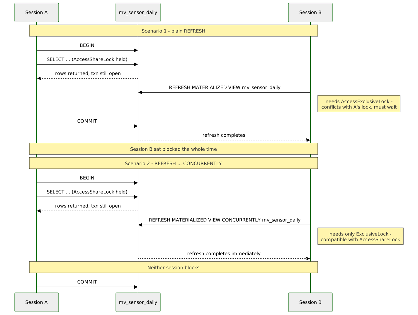
No wait, despite Session A’s transaction still being open.
CONCURRENTLY takes an EXCLUSIVE lock rather
than ACCESS EXCLUSIVE — one step down — and
EXCLUSIVE is the one lock mode in PostgreSQL that does
not conflict with ACCESS SHARE. Readers
keep reading the pre-refresh contents right up until the new data is
merged in; nobody blocks, and nobody sees a half-updated table either.
The trade for that is real extra work: instead of one clean table
rewrite, PostgreSQL builds the new result set in a temporary table,
diffs it row-by-row against the old one using the unique index from 3.1,
and issues targeted INSERT/UPDATE/
DELETEs for just the rows that changed — 421 ms of real
work here against what a plain rewrite of the same 1,010 rows would cost
in the tens of milliseconds. For a small rollup like this one, that
overhead is noise. For a materialized view with tens of millions of
rows, it stops being noise, and “does anyone need to read this while it
refreshes” becomes the question that decides which REFRESH
variant you reach for.
4.1 — A refresh script
#!/usr/bin/env bash
# refresh_daily.sh — nightly rollup refresh
psql -d portsmith -c "REFRESH MATERIALIZED VIEW CONCURRENTLY mv_sensor_daily;"chmod +x refresh_daily.sh
./refresh_daily.shREFRESH MATERIALIZED VIEW4.2 — Schedule it with OS-level cron
crontab -e0 2 * * * /home/chris/portsmith/refresh_daily.sh >> /var/log/portsmith_matview_refresh.log 2>&1Every night at 02:00, outside business hours, the rollup catches up
on whatever landed in sensor_readings during the day.
4.3 — Why this is the “poor man’s” version
This works, but it has the usual problems of anything scheduled
outside the database: it depends on a specific machine’s crontab
existing and being correct, its failures show up in a log file nobody’s
watching instead of a table you can query, and nothing stops two
overlapping runs if a refresh ever takes longer than the interval
between them. Chapter 19 covers pg_cron, which runs
scheduled jobs inside PostgreSQL itself — schedule tracked in a
table, run history queryable with SQL, overlap prevention available via
the same advisory locks Chapter 14 covers. Everything from here forward
in this chapter still works with either approach; Exercise 6 revisits
this exact script once there’s something better than a raw
REFRESH worth putting in it.
5.1 — Build the monthly view from the daily one, not from raw data
CREATE MATERIALIZED VIEW mv_sensor_monthly AS
SELECT
date_trunc('month', reading_day)::date AS reading_month,
sensor_type,
SUM(reading_count) AS reading_count,
round((SUM(avg_value * reading_count) / SUM(reading_count))::numeric, 2) AS avg_value,
round(MIN(min_value)::numeric, 2) AS min_value,
round(MAX(max_value)::numeric, 2) AS max_value
FROM mv_sensor_daily
GROUP BY 1, 2
WITH DATA;
CREATE UNIQUE INDEX idx_mv_sensor_monthly_month_type
ON mv_sensor_monthly (reading_month, sensor_type);SELECT 34
Time: 41.209 msTwo things worth noticing before moving on. First,
avg_value is computed as
SUM(avg_value * reading_count) / SUM(reading_count) — a
weighted average — not AVG(avg_value). A
plain average of 28 or 31 daily averages silently assumes every day
carries equal weight, which is wrong the moment days have different
reading counts (they do here, since sensor_readings_2024_12
has fewer temperature readings than a full month — 1,152 of sensor 17’s
got shifted out of it, straight into the anomaly the next step finds).
Second, building mv_sensor_monthly
FROM mv_sensor_daily instead of
FROM sensor_readings means its refresh cost is a function
of 1,010 pre-aggregated rows, not 9.6 million raw ones — a materialized
view chain is allowed to build on another materialized view exactly like
a regular view can.
5.2 — The row that shouldn’t be there
SELECT reading_month, sensor_type, reading_count, avg_value
FROM mv_sensor_monthly
ORDER BY reading_month DESC, sensor_type
LIMIT 3; reading_month | sensor_type | reading_count | avg_value
---------------+-------------+---------------+-----------
2025-12-01 | temperature | 1152 | 29.84
2024-12-01 | air_quality | 89280 | 34.51
2024-12-01 | temperature | 445248 | 41.02
(3 rows)A 2025-12-01 row, for one sensor type only, with a
suspiciously round 1,152-row count. This is Chapter 8’s sensor-17 clock
bug, now one layer removed from where it was first found: it landed in
sensor_readings, propagated automatically into
mv_sensor_daily as five stray 2025 dates, and propagated
automatically again into mv_sensor_monthly as a whole extra
month that shouldn’t exist on Portsmith’s 2024 dashboard. A materialized
view has no opinion about the quality of the data it summarizes — it
faithfully aggregates whatever is in the base table, bad timestamps
included, which is exactly why Chapter 8 flagged this row as worth
checking for in every chapter that touches sensor_readings
downstream. Any dashboard query built on mv_sensor_monthly
should filter to the expected year explicitly
(WHERE reading_month >= '2024-01-01' AND reading_month < '2025-01-01')
rather than assume the view only ever contains what it was “supposed”
to.

5.3 — Prove refreshes don’t cascade
Simulate a late-arriving reading — a traffic sensor that reported an hour behind schedule:
INSERT INTO sensor_readings (sensor_id, sensor_type, reading_value, recorded_at)
VALUES (51, 'traffic', 99, '2024-06-15 12:00:00+00');REFRESH MATERIALIZED VIEW CONCURRENTLY mv_sensor_daily;
SELECT reading_count FROM mv_sensor_daily
WHERE reading_day = '2024-06-15' AND sensor_type = 'traffic'; reading_count
---------------
11521mv_sensor_daily sees the new row — up from the usual
11,520. Now check the monthly view, without refreshing it:
SELECT reading_count FROM mv_sensor_monthly
WHERE reading_month = '2024-06-01' AND sensor_type = 'traffic'; reading_count
---------------
345600Still the old total. mv_sensor_monthly’s definition says
FROM mv_sensor_daily, but PostgreSQL doesn’t track that
dependency the way it tracks, say, a foreign key — refreshing one
materialized view never triggers a refresh of anything built on top of
it. It has to be done in order, explicitly:
REFRESH MATERIALIZED VIEW CONCURRENTLY mv_sensor_monthly;
SELECT reading_count FROM mv_sensor_monthly
WHERE reading_month = '2024-06-01' AND sensor_type = 'traffic'; reading_count
---------------
345601Now it matches. Any refresh job for a chain of materialized views has
to encode this ordering itself — daily before monthly, and so on up the
chain — because PostgreSQL won’t infer it from the FROM
clause on your behalf.
6.1 — Check what pg_matviews actually
tracks
It’s tempting to assume the catalog that lists materialized views also records when each one was last refreshed. Check directly:
\d pg_matviews View "pg_catalog.pg_matviews"
Column | Type | Collation | Nullable | Default
--------------+------+-----------+----------+---------
schemaname | name | | |
matviewname | name | | |
matviewowner | name | | |
tablespace | name | | |
hasindexes | boolean | | |
ispopulated | boolean | | |
definition | text | | |No timestamp, anywhere. ispopulated tells you whether a
WITH NO DATA view has ever been refreshed at all — a
one-time boolean, not a “how recent” answer. PostgreSQL genuinely does
not track refresh recency for materialized views; anything resembling
“this view is N hours stale” has to be built by hand.
6.2 — Build the tracking table and a helper to keep it honest
CREATE TABLE matview_refresh_log (
matview_name TEXT PRIMARY KEY,
refreshed_at TIMESTAMPTZ NOT NULL
);
CREATE OR REPLACE PROCEDURE refresh_and_log(p_matview regclass)
LANGUAGE plpgsql AS $$
BEGIN
EXECUTE format('REFRESH MATERIALIZED VIEW CONCURRENTLY %s', p_matview);
INSERT INTO matview_refresh_log (matview_name, refreshed_at)
VALUES (p_matview::text, clock_timestamp())
ON CONFLICT (matview_name) DO UPDATE SET refreshed_at = EXCLUDED.refreshed_at;
END;
$$;clock_timestamp() rather than now() —
now() is fixed for the whole transaction, and a
CALL to a procedure runs as one, so now()
would log the moment the procedure started, not the moment the
REFRESH inside it actually finished.
6.3 — Refresh both views through the tracked path
CALL refresh_and_log('mv_sensor_daily');
CALL refresh_and_log('mv_sensor_monthly');CALL
CALL6.4 — The staleness query
SELECT m.matviewname,
l.refreshed_at,
now() - l.refreshed_at AS age,
CASE
WHEN l.refreshed_at IS NULL THEN 'NEVER REFRESHED (untracked)'
WHEN now() - l.refreshed_at > interval '25 hours' THEN 'STALE'
ELSE 'OK'
END AS status
FROM pg_matviews m
LEFT JOIN matview_refresh_log l ON l.matview_name = m.matviewname
WHERE m.schemaname = 'public'
ORDER BY m.matviewname; matviewname | refreshed_at | age | status
--------------------+--------------------------------+----------------+--------
mv_sensor_daily | 2026-08-02 09:14:02.881204+00 | 00:00:04.113 | OK
mv_sensor_monthly | 2026-08-02 09:14:03.019552+00 | 00:00:03.975 | OK
(2 rows)The LEFT JOIN matters: a materialized view that was
created or refreshed by hand — bypassing refresh_and_log
entirely — shows up with a NULL refreshed_at
and the honest verdict “untracked,” rather than silently vanishing from
the report or falsely reading as fresh. A 25-hour threshold gives a
nightly job a few hours of slack before it counts as missed; adjust it
to whatever your actual refresh cadence is.
6.5 — Wire this back into Exercise 4’s cron job
#!/usr/bin/env bash
# refresh_daily.sh — nightly rollup refresh, now logged
psql -d portsmith -c "CALL refresh_and_log('mv_sensor_daily');"
psql -d portsmith -c "CALL refresh_and_log('mv_sensor_monthly');"Same crontab entry from 4.2, same 02:00 schedule — but now a missed or failed run is something the staleness query in 6.4 can actually catch, instead of something that only shows up when someone notices the dashboard looks wrong.
| Tool | What it does |
|---|---|
CREATE MATERIALIZED VIEW ... AS SELECT ... |
Runs a query once and stores the result as a real, indexable table |
WITH DATA / WITH NO DATA |
Populate immediately, or defer — an unpopulated view errors on
SELECT until refreshed |
pg_matviews.ispopulated |
Whether a view has ever been refreshed — a one-time flag, not a timestamp |
REFRESH MATERIALIZED VIEW |
Full rewrite under an ACCESS EXCLUSIVE lock — blocks
and is blocked by every reader |
REFRESH MATERIALIZED VIEW CONCURRENTLY |
Diff-based refresh under an EXCLUSIVE lock — doesn’t
block readers, but requires a unique index and costs more CPU/IO |
Matview chaining (FROM another matview) |
Legal and useful for cheap incremental rollups, but refreshes never cascade automatically |
matview_refresh_log +
refresh_and_log() |
The hand-built pattern for tracking refresh recency, since PostgreSQL doesn’t track it natively |
The key design insight from this chapter is that a
materialized view moves cost, it doesn’t remove it — every millisecond
Exercise 2 shaved off read time was paid for up front, at refresh time,
and the entire rest of the chapter is really about where that payment
lands. A plain REFRESH pays it in a lock that every reader
waits behind. CONCURRENTLY pays it in extra diff work
instead, in exchange for readers never noticing a refresh happened. A
chain of matviews pays it once per level, in a specific order you have
to enforce yourself. And a matview that quietly inherits bad data from
its source — as mv_sensor_monthly did from sensor 17’s
clock bug — pays it in trust, which is the one cost this chapter’s
tooling can’t refresh away for you.
Going further: sensor_readings still has more to
give. Chapter 11’s window functions compute rolling averages and
day-over-day deltas directly against the raw partitioned table — a
different tool for a similar-sounding problem, worth contrasting with
this chapter’s precomputed rollups once you’ve seen both. Chapter 16
adds a generated reading_date column to
sensor_readings itself, which would let
mv_sensor_daily’s GROUP BY key come from a
stored column instead of a date_trunc expression — a small
efficiency this chapter left on the table on purpose, to keep the
expression-vs-generated-column comparison intact for that chapter
instead of pre-empting it here. Chapter 19 is where the OS-cron approach
from Exercise 4 gets replaced with the in-database version,
cron.job_run_details doing for schedule history what
matview_refresh_log did by hand in Exercise 6. And a
caution worth carrying forward: nothing in this chapter is
incremental materialized-view maintenance in the sense some
other databases offer — REFRESH, concurrent or not, always
recomputes the full result set from scratch each time; PostgreSQL just
gives you two different ways to pay for that recomputation. Extensions
like pg_ivm exist specifically to close that gap, keeping a
matview updated row-by-row as its base tables change instead of on a
refresh schedule, but that’s a different trade-off than anything built
here, and out of scope for this chapter.
“PostgREST doesn’t generate an API from your schema. It is your schema, addressed over HTTP.”
Every chapter so far has ended at psql. Getting from “a
well-designed database” to “a web application that uses it” usually
means writing a backend: routes, an ORM layer, and — this is the part
that should sound familiar by now — a second, hand-written copy of the
authorization rules the database already enforces. A GRANT,
a CHECK constraint, a row level security policy: none of
that goes away when you add a web service, but it’s astonishingly common
to see it duplicated, in a different language, in application code that
can quietly drift out of sync with what the database actually
allows.
PostgREST removes the backend, not by hiding the database behind a
generated client SDK, but by putting the database directly on the wire.
It’s a single stateless binary that connects to PostgreSQL, introspects
the catalog, and turns every table and view it finds into a REST
resource and every function into an RPC endpoint. There is no PostgREST
authorization system to configure separately — a request arrives, an
HTTP verb and a role from a JWT decide what SQL statement to attempt, a
single transaction runs it as that role, and the same
GRANTs and RLS policies from every earlier chapter decide
whether it succeeds. The entire security model of this chapter is
Postgres roles you already know how to create.
That trade cuts both ways, and it’s worth naming up front: you get an API with no application code to audit, but you also get an API that can only do what a single SQL statement per request can do. There’s no middle-tier caching, no multi-step business logic spanning several tables outside of what a view or function can express, no background jobs. For Portsmith’s needs this chapter builds — a public directory, a permit intake form, a resident self-service lookup, a fuzzy search box — that’s not a limitation, it’s the entire point.
Portsmith’s small dev team wants four thin pieces of “app” without writing a backend for any of them:
Every one of these reuses a table this book already built. Nothing new gets seeded — Chapter 10 is entirely about exposing data, not generating it.
| Role | Purpose |
|---|---|
authenticator |
The only role PostgREST ever logs in as — NOINHERIT,
switches roles per request |
web_anon |
The public role — active whenever no JWT is presented |
web_resident |
Authenticated role for the resident portal, assumed via a JWT
role claim |
| Object | Purpose |
|---|---|
api.businesses |
Curated view over businesses (Chapter 1) — the public
directory |
api.jobs |
Curated view over jobs (Chapter 3) — permit intake |
api.residents |
Curated view over residents (Chapter 5) —
RLS-protected |
api.search_businesses() |
Wraps Chapter 5’s business_names trigram search as an
RPC endpoint |
By the end of this chapter you will be able to:
NOINHERIT role instead
of one role per API user.GET requests using
PostgREST’s query-parameter syntax, and read the
Content-Range header it returns.POST request against an
updatable view.GRANT/REVOKE, that PostgREST’s authorization
is really just PostgreSQL’s — no application code changes, no
restart.This chapter assumes PostgreSQL 16 is already running with the
businesses, jobs, and
residents/business_names tables in place — see
Loading the Data, below.
Debian doesn’t ship a current PostgREST package, and PostgREST’s own documentation recommends the prebuilt static binary over any distro package anyway — it’s a single file with no runtime dependencies. This chapter was written against v12.2 — check github.com/PostgREST/postgrest/releases for the current version and adjust the URL if a newer one exists:
curl -L -o postgrest.tar.xz \
https://github.com/PostgREST/postgrest/releases/download/v14.16/postgrest-v14.16-linux-static-x86-64.tar.xz
tar xJf postgrest.tar.xz
sudo mv postgrest /usr/local/bin/
rm postgrest.tar.xz
postgrest --help | head -3postgrest - Serve a RESTful API from any Postgres database
Usage: postgrest [-v|--version] [-e|--example]
[--dump-config | --dump-schema | --ready] [FILENAME]pyjwt, for
minting test tokenssource .venv/bin/activate
pip install pyjwtcurl and jqsudo apt install -y curl jqjq isn’t required, but every example below pipes through
| jq to keep the JSON readable — drop it if you’d rather
see raw output.
Nothing new to seed. This chapter needs Chapters 1, 3, and 5’s data to already exist:
python data/ch01_seed.py # businesses
python data/ch03_seed.py # jobs, dead_letter_jobs
python data/ch05_seed.py # residents, business_namesSELECT 'businesses' AS table, COUNT(*) FROM businesses
UNION ALL SELECT 'jobs', COUNT(*) FROM jobs
UNION ALL SELECT 'residents', COUNT(*) FROM residents
UNION ALL SELECT 'business_names', COUNT(*) FROM business_names; table | count
-----------------+-------
businesses | 48
jobs | 45
residents | 58
business_names | 48
(4 rows)If all four match, proceed to the exercises.
1.1 — The role PostgREST actually logs in as
PostgREST doesn’t map “one API caller” to “one Postgres login.” It
authenticates to Postgres exactly once, as a single low-privilege role,
and then uses SET ROLE inside each request’s transaction to
switch to whichever role the request is actually entitled to. That role
has to be NOINHERIT — otherwise it would automatically
carry the privileges of every role it can switch to, all the time,
defeating the entire point:
sudo -u postgres psql portsmithCREATE ROLE authenticator NOINHERIT LOGIN PASSWORD 'devsecret';
CREATE ROLE web_anon NOLOGIN;
CREATE ROLE web_resident NOLOGIN;
GRANT web_anon TO authenticator;
GRANT web_resident TO authenticator;web_anon and web_resident can never log in
directly (NOLOGIN) — they exist purely as identities
authenticator is allowed to become.
1.2 — A curated schema, not the raw tables
PostgREST exposes exactly the schema(s) you tell it to, and nothing
about db-schemas requires that schema to be
public. Building a separate api schema of
views — rather than pointing PostgREST straight at
businesses, jobs, and residents —
means the public-facing shape of the data can diverge from its internal
shape without either side having to know about the other’s
constraints:
CREATE SCHEMA IF NOT EXISTS api;
CREATE VIEW api.businesses AS
SELECT id,
name,
neighbourhood,
details ->> 'category' AS category,
(details ->> 'rating')::numeric AS rating
FROM businesses;
GRANT USAGE ON SCHEMA api TO web_anon, web_resident;
GRANT SELECT ON api.businesses TO web_anon;category and rating didn’t exist as real
columns anywhere — they’re pulled out of Chapter 1’s
details JSONB and given real, typed names. That’s a small
but genuine payoff from Chapter 1: the messy, schema-free column becomes
a clean, filterable, sortable API field, and the flexible storage and
the tidy public interface aren’t in tension with each other.
1.3 — postgrest.conf
db-uri = "postgres://authenticator:devsecret@localhost:5432/portsmith"
db-schemas = "api"
db-anon-role = "web_anon"
jwt-secret = "portsmith-lab-book-dev-secret-do-not-use-in-production"
db-channel-enabled = true
db-channel = "pgrst"
server-port = 3000db-anon-role is what authenticator becomes
for any request that doesn’t carry a valid JWT.
db-channel-enabled turns on LISTEN pgrst —
Exercise 3 uses it to tell a running PostgREST server about new views
without restarting it.
1.4 — Start it, and make one request
postgrest postgrest/postgrest.confListening on port 3000From another terminal:
curl -s "http://localhost:3000/businesses?limit=3" | jq[
{ "id": 1, "name": "The Gilded Clam", "neighbourhood": "Harbour District", "category": "restaurant", "rating": 4.5 },
{ "id": 2, "name": "Anchor & Oar Tavern", "neighbourhood": "Harbour District", "category": "restaurant", "rating": 4.1 },
{ "id": 3, "name": "Portsmith Fish Market", "neighbourhood": "Harbour District", "category": "retail", "rating": 4.8 }
]No route was written anywhere. /businesses exists
because api.businesses exists, db-schemas says
look in api, and web_anon has
SELECT on it. Delete the view and the route disappears with
it.
GET /businesses: Filter, Sort, Paginate2.1 — Filtering with eq, gte, and
friends
curl -s "http://localhost:3000/businesses?category=eq.restaurant&rating=gte.4.5&order=rating.desc&limit=5" | jq[
{ "id": 28, "name": "River Bend Bakery", "neighbourhood": "Riverside", "category": "restaurant", "rating": 4.8 },
{ "id": 11, "name": "Le Petit Bistro", "neighbourhood": "Old Town", "category": "restaurant", "rating": 4.7 },
{ "id": 10, "name": "Bella Napoli", "neighbourhood": "Old Town", "category": "restaurant", "rating": 4.6 },
{ "id": 31, "name": "Quay Street Deli", "neighbourhood": "Riverside", "category": "restaurant", "rating": 4.6 },
{ "id": 24, "name": "Spice Garden", "neighbourhood": "Northgate", "category": "restaurant", "rating": 4.6 }
]Every operator here — eq, gte,
order, limit — is a plain query parameter,
translated straight into a
WHERE/ORDER BY/LIMIT clause.
gte.4.5 reads almost like the SQL it becomes:
WHERE category = 'restaurant' AND rating >= 4.5.
2.2 — Paginating, and reading
Content-Range
curl -si "http://localhost:3000/businesses?category=eq.restaurant&order=name&limit=5&offset=5" \
-H "Prefer: count=exact" | head -20HTTP/1.1 206 Partial Content
Content-Range: 5-9/15
Content-Type: application/json; charset=utf-8
[
{ "id": 26, "name": "Mango Bay Caribbean", "neighbourhood": "Northgate", "category": "restaurant", "rating": 4.5 },
{ "id": 42, "name": "Port Canteen", "neighbourhood": "Industrial Port", "category": "restaurant", "rating": 3.7 },
{ "id": 31, "name": "Quay Street Deli", "neighbourhood": "Riverside", "category": "restaurant", "rating": 4.6 },
{ "id": 28, "name": "River Bend Bakery", "neighbourhood": "Riverside", "category": "restaurant", "rating": 4.8 },
{ "id": 25, "name": "Sol y Mar", "neighbourhood": "Northgate", "category": "restaurant", "rating": 4.3 }
]206 Partial Content and
Content-Range: 5-9/15 — rows 6 through 10 (0 indexed) out
of 15 restaurants total. Prefer: count=exact is what makes
PostgREST bother computing that total at all; without it, the
/15 is simply omitted, since counting the full match set
costs an extra query PostgREST won’t run unless asked. The same
pagination is also available as a Range: 5-9 request header
instead of limit/offset query parameters — two
spellings of the identical SQL.
2.3 — Narrowing columns with select
curl -s "http://localhost:3000/businesses?select=name,rating&neighbourhood=eq.Riverside&order=rating.desc" | jq[
{ "name": "River Bend Bakery", "rating": 4.8 },
{ "name": "Portsmith Veterinary Clinic", "rating": 4.8 },
{ "name": "Dr. Chen Dentistry", "rating": 4.7 },
{ "name": "The Art Depot", "rating": 4.6 },
{ "name": "Quay Street Deli", "rating": 4.6 }
]select maps directly onto the SELECT list —
the response body is exactly the columns asked for, never the whole row,
which matters once a client is fetching this over a slow connection or a
metered one.
POST /jobs: Filing a Permit Application3.1 — Expose the queue, add it to the running server
CREATE VIEW api.jobs AS
SELECT id, job_type, payload, priority, status, created_at
FROM jobs;
GRANT SELECT, INSERT ON api.jobs TO web_anon;api.jobs didn’t exist when PostgREST started, so it
isn’t in the server’s schema cache yet — a plain curl
against /jobs right now would 404. Tell the running server
to pick up the change, without restarting it:
NOTIFY pgrst, 'reload schema';3.2 — File a new permit application
curl -si -X POST "http://localhost:3000/jobs" \
-H "Content-Type: application/json" \
-H "Prefer: return=representation" \
-d '{
"job_type": "sign_permit",
"priority": 5,
"payload": {
"application_id": "SP-2024-0007",
"applicant_name": "Quay Street Deli",
"property_address": "31 Quay Street",
"neighbourhood": "Riverside",
"description": "New illuminated storefront sign",
"fee_due": 120.00
}
}'HTTP/1.1 401 Unauthorized
Content-Type: application/json; charset=utf-8
{"code":"42501","details":null,"hint":null,"message":"permission denied for sequence jobs_id_seq"}Not the response Exercise 3.1’s GRANT seemed to promise.
jobs.id is BIGSERIAL — shorthand for a
BIGINT column with
DEFAULT nextval('jobs_id_seq'), backed by a real sequence
object the table doesn’t own outright. The client never mentions
id in the request body, but Postgres still has to
call nextval() to fill in that default while
executing the INSERT, and calling a sequence requires its
own USAGE privilege — separate from, and not implied by,
INSERT on the table or view sitting on top of it.
GRANT INSERT alone is never enough for a table whose
primary key is
SERIAL/BIGSERIAL/IDENTITY:
GRANT USAGE ON SEQUENCE jobs_id_seq TO web_anon;3.3 — Retry
curl -si -X POST "http://localhost:3000/jobs" \
-H "Content-Type: application/json" \
-H "Prefer: return=representation" \
-d '{
"job_type": "sign_permit",
"priority": 5,
"payload": {
"application_id": "SP-2024-0007",
"applicant_name": "Quay Street Deli",
"property_address": "31 Quay Street",
"neighbourhood": "Riverside",
"description": "New illuminated storefront sign",
"fee_due": 120.00
}
}'HTTP/1.1 201 Created
Content-Type: application/json; charset=utf-8
[
{
"id": 46, "job_type": "sign_permit", "priority": 5,
"payload": { "application_id": "SP-2024-0007", "applicant_name": "Quay Street Deli", ... },
"status": "queued", "created_at": "2026-08-02T09:41:07.221Z"
}
]No client-supplied id, status, or
created_at — all three came from the table’s own defaults,
exactly as they would from a plain INSERT missing those
columns. Prefer: return=representation is what makes
PostgREST hand the created row back at all; without it, a successful
POST returns 201 with an empty body and a
Location header instead. This job now sits in the same
jobs table Chapter 3’s FOR UPDATE SKIP LOCKED
workers claim from — the web request and the queue worker never have to
know about each other.
4.1 — The grant from Exercise 3 is looser than it looks
GRANT INSERT ON api.jobs gave web_anon
permission to set every column in the view — including
status. Nothing stops a client from walking straight past
“submitted” and declaring their own application already approved:
curl -si -X POST "http://localhost:3000/jobs" \
-H "Content-Type: application/json" \
-H "Prefer: return=representation" \
-d '{"job_type": "sign_permit", "priority": 5, "payload": {"application_id": "SP-2024-0008"}, "status": "completed"}'HTTP/1.1 201 Created
[{ "id": 47, "job_type": "sign_permit", "priority": 5, "payload": {...}, "status": "completed", "created_at": "..." }]That succeeded, and it shouldn’t have — a permit that was never
reviewed now reads as completed, indistinguishable in the
queue from one Chapter 3’s worker actually finished. Nothing in
PostgREST’s configuration causes this; it’s a plain over-broad
GRANT, the same mistake it would be in any hand-written
backend.
4.2 — Fix it with a column-level grant
REVOKE INSERT ON api.jobs FROM web_anon;
GRANT INSERT (job_type, payload, priority) ON api.jobs TO web_anon;PostgreSQL’s INSERT privilege can be scoped to specific
columns, not just the whole table. web_anon can now insert
a row, but only by supplying values for these three columns — every
other column must come from its default.
4.3 — The same malicious request, after the grant change
curl -si -X POST "http://localhost:3000/jobs" \
-H "Content-Type: application/json" \
-d '{"job_type": "sign_permit", "priority": 5, "payload": {"application_id": "SP-2024-0009"}, "status": "completed"}'HTTP/1.1 401 Unauthorized
Content-Type: application/json; charset=utf-8
{"code":"42501","details":null,"hint":null,"message":"permission denied for table jobs"}401, not 403 — PostgREST reserves
403 for a request that authenticated as someone
and was still refused; an unauthenticated request denied by the database
gets 401, the same “you may need to log in for this” signal
a browser would show for any other protected resource. No PostgREST
config changed between 4.1 and 4.3, and the server was never restarted —
only a database GRANT changed, and the API’s behavior
changed the instant that transaction committed, because PostgREST never
cached a decision about it in the first place.
4.4 — The legitimate request still works
curl -si -X POST "http://localhost:3000/jobs" \
-H "Content-Type: application/json" \
-H "Prefer: return=representation" \
-d '{"job_type": "sign_permit", "priority": 5, "payload": {"application_id": "SP-2024-0009", "applicant_name": "Old Town Hardware", "fee_due": 95.00}}'HTTP/1.1 201 Created
[{ "id": 48, "job_type": "sign_permit", "priority": 5, "payload": {...}, "status": "queued", "created_at": "..." }]Omit status entirely and the table’s own
DEFAULT 'queued' fills it in, exactly like Exercise 3 — the
column-level grant didn’t break the honest use case, it just closed off
the dishonest one.
residents5.1 — Expose residents, but to nobody yet
CREATE VIEW api.residents WITH (security_invoker = true) AS
SELECT id, full_name, neighbourhood
FROM residents;true_duplicate_of — Chapter 5’s ground-truth column for
grading the fuzzy-matching exercises — is deliberately left out. It’s
exactly the kind of internal bookkeeping column a curated view exists to
hide from the outside world.
security_invoker = true is not optional here, and
skipping it is the kind of mistake that only shows up once you’re
testing with two different JWTs and notice neither one got filtered. By
default, a view runs with the privileges of whoever owns it,
not whoever is querying it — including, critically, for deciding which
row security policies apply. That default is normally a feature: it’s
exactly what lets web_anon, which has no direct grant on
businesses at all, read anything through
api.businesses. But every object in this chapter was
created from the sudo -u postgres psql session back in
Exercise 1.1, which makes postgres — a superuser — the
owner of api.residents. Superusers bypass row level
security unconditionally, no exceptions. Left at its default, this view
would evaluate Exercise 5.2’s policy as postgres on every
single request, regardless of which role or JWT actually called it, and
a bypassed policy filters nothing — every resident would see every row.
security_invoker = true makes the view check privileges and
RLS as the real caller instead: web_resident, after
PostgREST’s per-request SET ROLE, exactly as Exercise 5.2’s
policy expects.
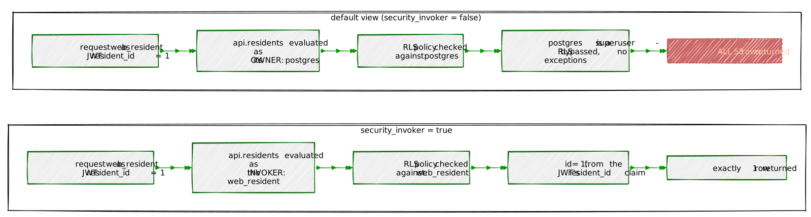
(If you’re changing an existing view rather than creating
this one fresh, reach for
ALTER VIEW api.residents SET (security_invoker = true);
instead of dropping and recreating it — DROP VIEW followed
by CREATE VIEW makes a brand-new object with none of the
original’s grants, so Exercise 5.2’s
GRANT SELECT ON api.residents TO web_resident would
silently need to be re-run, and the endpoint would 403 with
permission denied for view residents until it is.)
NOTIFY pgrst, 'reload schema';No GRANT yet, on purpose — not even to
web_resident. RLS goes on before any role can read a single
row.
5.2 — Enable RLS and add a self-only policy
ALTER TABLE residents ENABLE ROW LEVEL SECURITY;
CREATE POLICY resident_self_only ON residents
FOR SELECT
USING (id = (current_setting('request.jwt.claims', true)::json ->> 'resident_id')::int);
GRANT SELECT ON api.residents TO web_resident;
GRANT SELECT (id, full_name, neighbourhood) ON residents TO web_resident;current_setting('request.jwt.claims', true) reads the
JSON claims object PostgREST sets, per request, from the caller’s
verified JWT — the true second argument means “return NULL
instead of erroring if it’s unset,” which matters because
web_anon requests never carry one at all. The policy
compares the row’s own id against whatever
resident_id claim a valid, signed JWT presents.
Both GRANTs are required, and it’s easy to stop at the
first one and not notice. security_invoker = true from
Exercise 5.1 means api.residents no longer borrows its
owner’s privileges to read the underlying table — the invoking role
needs real privileges of its own on residents, not just on
the view sitting in front of it. Skip the second GRANT and
every request fails with
permission denied for table residents, even though the role
clearly has SELECT on the view; the view-level check
passes, and the query still dies one level down, on the base table it
was never given access to. The column list
(id, full_name, neighbourhood) matters too, not just the
table name: granting only these three columns — matching exactly what
api.residents selects — keeps
true_duplicate_of unreachable even if
web_resident were ever queried against directly instead of
through the view, which a bare GRANT SELECT ON residents
(no column list) would not.
5.3 — Mint a JWT per resident
#!/usr/bin/env python3.12
# mint_jwt.py — issue a dev-only resident session token
import sys
import jwt
SECRET = "portsmith-lab-book-dev-secret-do-not-use-in-production"
resident_id = int(sys.argv[1])
token = jwt.encode(
{"role": "web_resident", "resident_id": resident_id},
SECRET,
algorithm="HS256",
)
print(token)The role claim is what PostgREST uses to decide which
role to SET ROLE to for this request — it has to be a role
authenticator was granted membership in back in Exercise
1.1, or PostgREST refuses the token outright.
5.4 — Two residents, two different answers from the same endpoint
TOKEN_1=$(python mint_jwt.py 1) # Adrian Foscolo
TOKEN_2=$(python mint_jwt.py 2) # Marisol Quintero
curl -s "http://localhost:3000/residents" -H "Authorization: Bearer $TOKEN_1" | jq
curl -s "http://localhost:3000/residents" -H "Authorization: Bearer $TOKEN_2" | jq[ { "id": 1, "full_name": "Adrian Foscolo", "neighbourhood": "Old Town" } ][ { "id": 2, "full_name": "Marisol Quintero", "neighbourhood": "Riverside" } ]Identical request, identical route, identical GRANT —
the only difference is which JWT signed it, and RLS silently rewrote
each query’s effective WHERE clause to match.
5.5 — The gotcha: RLS filters, it doesn’t refuse
curl -s "http://localhost:3000/residents?id=eq.2" -H "Authorization: Bearer $TOKEN_1" | jq[]Resident 1, asking directly for resident 2’s row by id, does
not get a 403 — they get
200 OK and an empty array. This is a meaningfully different
failure mode from Exercise 4’s column-privilege denial: a
GRANT violation is an error, loud and explicit; an RLS
mismatch is just a WHERE clause that happens to match
nothing, indistinguishable at the HTTP layer from “that id doesn’t
exist.” Compare with no credentials at all:
curl -si "http://localhost:3000/residents"HTTP/1.1 401 Unauthorized
{"code":"42501","details":null,"hint":null,"message":"permission denied for table residents"}This one errors, the same way Exercise 4.3 did —
web_anon was never granted SELECT on
api.residents at all, so it never gets far enough to run
into the RLS policy in the first place. Two different denials, two
different HTTP shapes, and the difference between them is worth being
able to explain: a missing GRANT is a wall; RLS is a
filter.
6.1 — Wrap Chapter 5’s trigram search as a function
CREATE OR REPLACE FUNCTION api.search_businesses(search_term text)
RETURNS TABLE (business_id integer, name text, similarity numeric)
LANGUAGE sql STABLE AS $$
SELECT business_id, name, round(similarity(name, search_term)::numeric, 3) AS similarity
FROM business_names
ORDER BY name <-> search_term
LIMIT 5;
$$;
GRANT EXECUTE ON FUNCTION api.search_businesses(text) TO web_anon;
GRANT SELECT ON business_names TO web_anon;NOTIFY pgrst, 'reload schema';The function body is Chapter 5, Exercise 5’s exact “did you mean?”
query, verbatim — name <-> search_term ordering by
trigram distance, backed by the
idx_business_names_trgm_gist GiST index that chapter built.
PostgREST doesn’t need to know anything about trigrams; it just sees a
function in the api schema and exposes it at
/rpc/.
Both GRANTs are required, for the same reason Exercise
5.2 needed two of them. SQL functions default to
SECURITY INVOKER — this one was never told otherwise — so
api.search_businesses() runs its
SELECT ... FROM business_names as whichever role actually
called it, web_anon here, not as the function’s owner.
EXECUTE only grants permission to call the
function; it says nothing about what the function is allowed to touch
once it’s running. Skip the second GRANT and 6.2 fails with
permission denied for table business_names,
EXECUTE privilege notwithstanding — the same wall Exercise
5.2 hit with residents, just one function-call away instead
of one view away.
6.2 — Call it
curl -s -X POST "http://localhost:3000/rpc/search_businesses" \
-H "Content-Type: application/json" \
-d '{"search_term": "Ironsyde Auto"}' | jq[
{ "business_id": 45, "name": "Ironside Auto", "similarity": 0.647 },
{ "business_id": 21, "name": "AutoFix Portsmith", "similarity": 0.143 },
{ "business_id": 4, "name": "Harbour Inn", "similarity": 0.040 },
{ "business_id": 36, "name": "The Art Depot", "similarity": 0.037 },
{ "business_id": 34, "name": "Riverside Cinema", "similarity": 0.033 }
]Same misspelling, same top match, same scores as Chapter 5’s own
psql session — this endpoint is that query, not a
reimplementation of it.
6.3 — GET works too, because the function is
STABLE
curl -s "http://localhost:3000/rpc/search_businesses?search_term=Ironsyde+Auto" | jq -c '.[0]'{"business_id":45,"name":"Ironside Auto","similarity":0.647}PostgREST maps a function’s SQL volatility onto which HTTP verbs it
will accept: VOLATILE functions — anything that could
plausibly write data — are reachable only by POST, on the
theory that a GET should always be safe to retry, cache, or
prefetch without side effects. STABLE and
IMMUTABLE functions, like this one, are exposed under both
GET and POST, because Postgres itself already
promises they don’t change anything. Declaring
LANGUAGE sql STABLE back in 6.1 wasn’t just documentation —
it’s the line that decided whether a browser could ever call this
endpoint from a plain link.
Every real failure in this chapter — Exercise 3’s
jobs_id_seq, Exercise 5’s residents columns,
this exercise’s business_names — turned out to be the same
shape: one grant in place, a second, independent one missing, one layer
further in than the error first suggests:
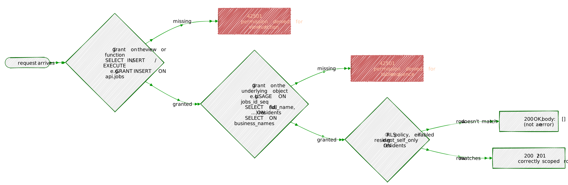
| Tool | What it does |
|---|---|
authenticator role, NOINHERIT |
The one role PostgREST logs in as; switches per-request via
SET ROLE |
db-anon-role |
The role a request without a valid JWT runs as |
api schema of views |
Decouples the public API shape from the internal table shape |
NOTIFY pgrst, 'reload schema' |
Tells a running PostgREST server about new tables/views/functions without a restart |
?col=eq.x, ?order=, ?select=,
?limit=/?offset= |
Query-parameter syntax mapping directly onto
WHERE/ORDER BY/SELECT/LIMIT |
Prefer: return=representation |
Get the affected row(s) back in the response body |
Prefer: count=exact / Content-Range |
Ask for, and read, the total row count behind a paginated result |
Column-level GRANT/REVOKE |
Restrict which fields a client can set on INSERT,
enforced by Postgres itself |
GRANT USAGE ON SEQUENCE ... |
Needed alongside INSERT for any
SERIAL/BIGSERIAL/IDENTITY
column’s default nextval() to succeed — table privileges
don’t imply sequence privileges |
401 vs. 403 |
401 = denied and unauthenticated (or bad JWT);
403 = denied despite valid credentials |
RLS policy vs. missing GRANT |
RLS silently filters rows (still 200, possibly empty);
a missing grant is a hard error |
security_invoker = true on a view |
Makes the view check privileges and RLS as the querying role, not the view’s owner — required for RLS to mean anything through a view owned by a superuser or the table owner |
/rpc/<function> |
A SQL function exposed as an endpoint; GET-eligible
only if STABLE/IMMUTABLE |
The key design insight from this chapter is that
every access-control decision PostgREST makes was already something
PostgreSQL could do — this chapter never introduced a new authorization
concept, only a new transport for reaching decisions the database was
always capable of making. GRANT/REVOKE from
Exercise 4 and row level security from Exercise 5 aren’t PostgREST
features with database-flavored names; they are exactly the
GRANT and CREATE POLICY you’d write for any
other purpose, and PostgREST’s only job was to authenticate a request,
pick a role, and get out of the way. That’s also this chapter’s sharpest
limitation, in the same sentence: anything that can’t be expressed as
one role running one SQL statement — multi-step workflows, calling
another API mid-request, anything genuinely procedural — is out of scope
by design, not by oversight.
Going further: Chapter 13’s
LISTEN/NOTIFY is the same primitive this
chapter used for schema-reload notifications, applied to application
data instead — a natural next step once
NOTIFY pgrst, 'reload schema' feels familiar. Chapter 14’s
advisory locks are worth knowing about if an RPC function like
api.search_businesses() ever needs to serialize access to a
shared resource instead of just reading one. And the column-level
GRANT from Exercise 4 generalizes: PostgreSQL’s full
privilege system — SELECT, UPDATE, and
REFERENCES privileges can all be scoped per-column the same
way INSERT was here — is worth a deliberate read through
the GRANT documentation before exposing any table this way
for real, well beyond what one chapter’s exercises can cover.
GROUP BY“
GROUP BYanswers a question by throwing away the rows that don’t fit in the answer. A window function answers the same question and keeps every row anyway.”
If you’ve used GROUP BY, you already know the shape of
the problem this chapter solves — and the shape of its one real
limitation. GROUP BY answers “what’s the average rating per
neighbourhood?” by collapsing every business in a neighbourhood down
into a single output row: you get the average, but every individual
business that went into computing it is gone from the result. Most of
the time that’s exactly what you want. But plenty of real questions
don’t fit that shape: “how does each business’s rating compare to its
neighbourhood’s average, while still showing me every
business?” “What’s this business’s running revenue total, quarter
by quarter, without collapsing the quarters together?”
GROUP BY cannot answer either one — the instant it groups,
the individual rows that made up the group are gone for good.
A window function answers a
GROUP BY-shaped question without paying that price. It
looks at a set of rows related to the current row — its “window” —
computes something over them, and attaches the result to the current
row, which survives, completely unchanged, right alongside every other
row. Nothing collapses. Start with 48 rows, end with 48 rows, every one
of them now carrying an answer that depended on looking at some of its
neighbours.
That’s the single idea this entire chapter builds on, and it’s worth sitting with before touching any syntax:
GROUP BYreduces row count. A window function never does.
Every example below is built from four ingredients. Knowing what each one means in plain language first should make the SQL read as sentences instead of unfamiliar syntax:
| Piece | Plain-language meaning |
|---|---|
OVER (...) |
“Compute this using a window of related rows, not just this one
row.” Attached after a function call — AVG(x) OVER (...) —
it’s what turns an ordinary aggregate into a window function. An empty
OVER () means “the window is every row in the result.” |
PARTITION BY col |
“Only look at rows that share this row’s value of col.”
The window equivalent of GROUP BY — it restricts which
rows count, without collapsing any of them. |
ORDER BY col (written inside
OVER (...)) |
“Put the rows in this order before computing.” This ordering lives
entirely inside the window — it’s unrelated to the query’s own outer
ORDER BY, and the two are free to differ or even
conflict. |
frame clause —
e.g. ROWS BETWEEN 6 PRECEDING AND CURRENT ROW |
Out of the rows the partition and ordering make available, exactly which ones count toward this specific row’s calculation. |
Exercise 1 walks through all four, one at a time, against a dataset small enough to check by hand — five numbers, no Portsmith backstory required, so the mechanics stay in view before any real data shows up.
This chapter doesn’t tell one Portsmith story — it reuses four different tables to show that window functions are a general-purpose tool, not a feature tied to any one kind of data:
| Object | Source | Used for |
|---|---|---|
businesses |
Chapter 1 | Ranking businesses within their own neighbourhood |
sensor_readings |
Chapter 8 | 7-day rolling averages and day-over-day change |
network_events |
Chapter 7 | Detecting login “sessions” via gaps and islands |
business_revenue |
(new, this chapter) | Running totals and percentage-of-category-total |
business_revenue is the one genuinely new thing here — a
small, synthetic quarterly revenue figure for each of the 48 businesses
from Chapter 1, built specifically so Exercise 6 has real running-total
and percentage-of-partition data to work with.
By the end of this chapter you will be able to:
AVG(x) OVER () returns a value on every row while
AVG(x) with GROUP BY returns one row — and
predict, for any OVER (...) clause, exactly which rows are
“in the window” for a given output row.RANK() and
DENSE_RANK(), and state precisely how the two disagree the
moment there’s a tie.ORDER BY to a window — with no frame
clause at all — silently changes the default frame.LAG()/LEAD() to compare a row to its
neighbour without a self-join.PARTITION BY scopes — one for a
running total, one for a percentage-of-total — in a single
SELECT.Nothing to install. Window functions have been part of core PostgreSQL since version 8.4 (2009) — no extension, no configuration.
This chapter needs Chapters 1, 7, and 8’s data, plus one new small table:
python data/ch01_seed.py # businesses
python data/ch07_seed.py # network_events
python data/ch08_seed.py # sensors, then run Chapter 8's own exercises
# through Exercise 2 to get sensor_readings populated
python data/ch11_seed.py # business_revenue (new this chapter)business_revenue only needs businesses to
already exist — it doesn’t depend on Chapters 7 or 8 at all.
SET timezone = 'UTC';Same reason as Chapter 8: Exercises 3 and 4 group
sensor_readings by
date_trunc('day', recorded_at), and a day boundary computed
in any timezone other than UTC quietly buckets a different set of
5-minute readings into “Feb 1” than the ones this chapter’s numbers were
computed from — not a rounding difference, a genuinely different
average, since each bucket ends up averaging different rows entirely.
Run this at the top of every session in this chapter, including the psql
session that runs the prerequisite check below, or Exercises 3 and 4’s
numbers won’t match what’s printed here even though the query is
identical.
SELECT 'businesses' AS table, COUNT(*) FROM businesses
UNION ALL SELECT 'network_events', COUNT(*) FROM network_events
UNION ALL SELECT 'sensor_readings', COUNT(*) FROM sensor_readings
UNION ALL SELECT 'business_revenue', COUNT(*) FROM business_revenue; table | count
--------------------+---------
businesses | 48
network_events | 116
sensor_readings | 9648000
business_revenue | 192
(4 rows)If all four match, proceed to the exercises.
Forget Portsmith for a moment. Here are five temperature readings from one morning:
SELECT * FROM (VALUES
('06:00'::time, 52.1),
('07:00'::time, 53.4),
('08:00'::time, 55.8),
('09:00'::time, 58.2),
('10:00'::time, 60.5)
) AS t(reading_time, temp_f); reading_time | temp_f
--------------+--------
06:00:00 | 52.1
07:00:00 | 53.4
08:00:00 | 55.8
09:00:00 | 58.2
10:00:00 | 60.5
(5 rows)Five rows in, five rows to reason about. Keep this exact dataset in mind for everything below.
1.1 — GROUP BY collapses; OVER ()
doesn’t
SELECT AVG(temp_f) FROM (VALUES
('06:00'::time, 52.1), ('07:00'::time, 53.4), ('08:00'::time, 55.8),
('09:00'::time, 58.2), ('10:00'::time, 60.5)
) AS t(reading_time, temp_f); avg
---------------------
56.0000000000000000
(1 row)Five rows go in, one number comes out. That’s the
AVG(temp_f) you already know. Now the window version — same
aggregate, same result, one difference:
SELECT reading_time, temp_f,
round(AVG(temp_f) OVER ()::numeric, 2) AS morning_avg
FROM (VALUES
('06:00'::time, 52.1), ('07:00'::time, 53.4), ('08:00'::time, 55.8),
('09:00'::time, 58.2), ('10:00'::time, 60.5)
) AS t(reading_time, temp_f); reading_time | temp_f | morning_avg
--------------+--------+-------------
06:00:00 | 52.1 | 56.00
07:00:00 | 53.4 | 56.00
08:00:00 | 55.8 | 56.00
09:00:00 | 58.2 | 56.00
10:00:00 | 60.5 | 56.00
(5 rows)Five rows go in, five rows come out — every one of them now carrying
56.00, the exact number GROUP BY gave you,
just not at the cost of the other four rows. An empty
OVER () means “the window is every row here,” so every row
gets the same whole-set average stamped onto it. This is the entire idea
from the Background section, now sitting in front of you as actual
output: nothing collapsed.
1.2 — The gotcha: adding ORDER BY silently
changes the frame
Now add one thing — ORDER BY reading_time,
inside the OVER (...):
SELECT reading_time, temp_f,
round(AVG(temp_f) OVER (ORDER BY reading_time)::numeric, 2) AS running_avg
FROM (VALUES
('06:00'::time, 52.1), ('07:00'::time, 53.4), ('08:00'::time, 55.8),
('09:00'::time, 58.2), ('10:00'::time, 60.5)
) AS t(reading_time, temp_f); reading_time | temp_f | running_avg
--------------+--------+-------------
06:00:00 | 52.1 | 52.10
07:00:00 | 53.4 | 52.75
08:00:00 | 55.8 | 53.77
09:00:00 | 58.2 | 54.88
10:00:00 | 60.5 | 56.00
(5 rows)Same function, same data, completely different numbers — and only the
last row still shows 56.00. This is the single
most common surprise in all of window functions, so it’s worth tracing
exactly what changed, row by row:
reading_time |
temp_f |
rows actually included in this row’s window | running_avg |
|---|---|---|---|
| 06:00 | 52.1 | [06:00] |
52.10 |
| 07:00 | 53.4 | [06:00, 07:00] |
52.75 |
| 08:00 | 55.8 | [06:00, 07:00, 08:00] |
53.77 |
| 09:00 | 58.2 | [06:00, 07:00, 08:00, 09:00] |
54.88 |
| 10:00 | 60.5 | [06:00, 07:00, 08:00, 09:00, 10:00] |
56.00 |
Adding ORDER BY to a window did not just sort the rows —
it silently changed how many rows count for each one, from
“every row” down to “every row up to and including this one.” That’s
PostgreSQL’s default frame the moment a window has an
ORDER BY and no explicit frame clause:
RANGE UNBOUNDED PRECEDING AND CURRENT ROW, i.e., a running
calculation. Without ORDER BY, there’s nothing to run
up to, so the default frame is the whole partition instead,
which is exactly what 1.1’s flat 56.00 was. Nothing in the
syntax announces this change — ORDER BY looks like it
should only affect display order, and inside a window it affects
something much bigger. Committing this one rule to memory now will save
you from debugging a “wrong” running total later that was never actually
wrong, just unexpectedly running.
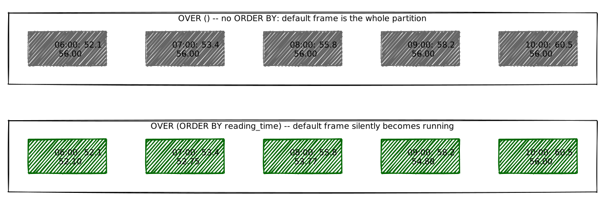
1.3 — PARTITION BY: independent windows, still
no collapsing
Add a second sensor to the tiny dataset:
SELECT sensor_label, reading_time, temp_f,
round(AVG(temp_f) OVER (PARTITION BY sensor_label ORDER BY reading_time)::numeric, 2) AS running_avg
FROM (VALUES
('Temp-01', '06:00'::time, 52.1), ('Temp-01', '07:00'::time, 53.4), ('Temp-01', '08:00'::time, 55.8),
('Temp-02', '06:00'::time, 48.9), ('Temp-02', '07:00'::time, 49.5), ('Temp-02', '08:00'::time, 50.1)
) AS t(sensor_label, reading_time, temp_f)
ORDER BY sensor_label, reading_time; sensor_label | reading_time | temp_f | running_avg
--------------+--------------+--------+-------------
Temp-01 | 06:00:00 | 52.1 | 52.10
Temp-01 | 07:00:00 | 53.4 | 52.75
Temp-01 | 08:00:00 | 55.8 | 53.77
Temp-02 | 06:00:00 | 48.9 | 48.90
Temp-02 | 07:00:00 | 49.5 | 49.20
Temp-02 | 08:00:00 | 50.1 | 49.50Temp-01‘s running average never sees
Temp-02’s numbers, and vice versa —
PARTITION BY walled the two sensors off into completely
independent windows, the same way GROUP BY sensor_label
would have, except both sensors’ six rows are all still here. This is
PARTITION BY doing to a window exactly what it would do to
a GROUP BY: split the data into groups — just without ever
throwing a row away.
1.4 — An explicit frame clause: precise control
1.2’s running average grows to include more and more history as it goes — by the last row, it’s averaging all five readings. A rolling average instead asks “the last N readings only,” which needs an explicit frame clause instead of relying on the default:
SELECT reading_time, temp_f,
round(AVG(temp_f) OVER (ORDER BY reading_time
ROWS BETWEEN 1 PRECEDING AND CURRENT ROW)::numeric, 2) AS rolling_2
FROM (VALUES
('06:00'::time, 52.1), ('07:00'::time, 53.4), ('08:00'::time, 55.8),
('09:00'::time, 58.2), ('10:00'::time, 60.5)
) AS t(reading_time, temp_f); reading_time | temp_f | rolling_2
--------------+--------+-----------
06:00:00 | 52.1 | 52.10
07:00:00 | 53.4 | 52.75
08:00:00 | 55.8 | 54.60
09:00:00 | 58.2 | 57.00
10:00:00 | 60.5 | 59.35reading_time |
rows in this row’s window
(1 PRECEDING AND CURRENT ROW) |
rolling_2 |
|---|---|---|
| 06:00 | [06:00] — no prior row exists yet, so just itself |
52.10 |
| 07:00 | [06:00, 07:00] |
52.75 |
| 08:00 | [07:00, 08:00] |
54.60 |
| 09:00 | [08:00, 09:00] |
57.00 |
| 10:00 | [09:00, 10:00] |
59.35 |
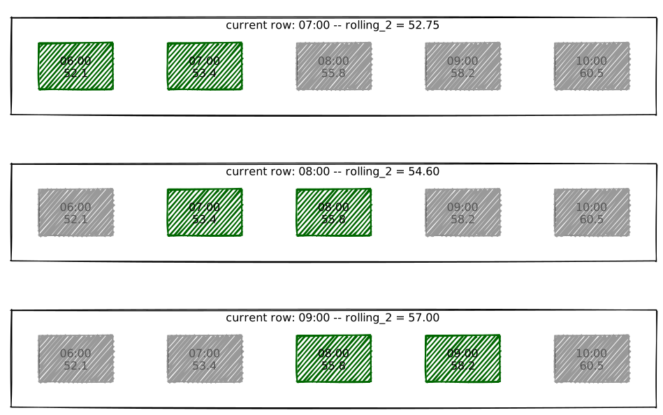
The window is now a fixed-size sliding pair, not an ever-growing
history — 08:00’s value depends on 07:00 and
08:00 only, never 06:00.
ROWS BETWEEN 1 PRECEDING AND CURRENT ROW is deliberately
the same shape of clause Exercise 3 uses next, just with a smaller
number: this tiny example is a 2-reading rolling average, and
Exercise 3 is nothing more than this same idea with
6 PRECEDING and real sensor data behind it.
2.1 — RANK() and DENSE_RANK(), side
by side
SELECT name, neighbourhood, (details->>'rating')::numeric AS rating,
RANK() OVER (PARTITION BY neighbourhood ORDER BY (details->>'rating')::numeric DESC) AS rank,
DENSE_RANK() OVER (PARTITION BY neighbourhood ORDER BY (details->>'rating')::numeric DESC) AS dense_rank
FROM businesses
WHERE neighbourhood IN ('Harbour District', 'Riverside')
ORDER BY neighbourhood, rating DESC; name | neighbourhood | rating | rank | dense_rank
------------------------------+------------------+--------+------+------------
Lighthouse Bookshop | Harbour District | 5.0 | 1 | 1
Portsmith Fish Market | Harbour District | 4.8 | 2 | 2
Saltbox Gallery | Harbour District | 4.7 | 3 | 3
Mariners Rest B&B | Harbour District | 4.7 | 3 | 3
Harbour View Theater | Harbour District | 4.6 | 5 | 4
Tidal Wave Surf Shop | Harbour District | 4.5 | 6 | 5
The Gilded Clam | Harbour District | 4.5 | 6 | 5
Harbour Inn | Harbour District | 4.3 | 8 | 6
Anchor & Oar Tavern | Harbour District | 4.1 | 9 | 7
River Bend Bakery | Riverside | 4.8 | 1 | 1
Portsmith Veterinary Clinic | Riverside | 4.8 | 1 | 1
Dr. Chen Dentistry | Riverside | 4.7 | 3 | 2
Quay Street Deli | Riverside | 4.6 | 4 | 3
The Art Depot | Riverside | 4.6 | 4 | 3
Thai Orchid | Riverside | 4.5 | 6 | 4
The Riverside Vegan | Riverside | 4.5 | 6 | 4
Riverside Cinema | Riverside | 4.4 | 8 | 5
Portsmith Pharmacy | Riverside | 4.3 | 9 | 6
(18 rows)(Lighthouse Bookshop’s 5.0 is Chapter 1,
Exercise 5’s jsonb_set update — if you’re seeing
4.9 instead, that exercise hasn’t run yet in this database,
which is fine; the ranking logic below is identical either way.)
2.2 — Reading the tie exactly
Look at Harbour District’s two businesses tied at 4.7:
both get rank = 3. The next business down, at
4.6, gets rank = 5 under RANK() —
4 is simply never used, because two rows already claimed
“3rd place” and RANK() counts every row ahead of you, ties
included. DENSE_RANK() disagrees on principle: it counts
distinct rating values seen so far, so 4.6 is the
4th distinct value in the list and gets dense_rank = 4, no
gap. Neither is “more correct” — RANK() answers “how many
businesses rate at or above me,” DENSE_RANK() answers “how
many distinct rating tiers are at or above me” — but they give a
different answer to “who’s in 4th place” the moment any tie exists, and
Riverside’s 4.8 tie two rows later shows the same split
happening again.
sensor_readings3.1 — Aggregate to daily first
sensor_readings reports every five minutes — a rolling
average over raw readings would be a rolling average of noise. Roll up
to one row per day first, the same shape of query Chapter 9 turned into
a materialized view, just computed directly here instead:
WITH daily AS (
SELECT date_trunc('day', recorded_at)::date AS reading_day,
round(AVG(reading_value)::numeric, 2) AS daily_avg
FROM sensor_readings
WHERE sensor_id = 1
AND recorded_at >= '2024-02-01' AND recorded_at < '2024-02-15'
GROUP BY 1
)
SELECT * FROM daily ORDER BY reading_day; reading_day | daily_avg
-------------+-----------
2024-02-01 | 42.46
2024-02-02 | 42.37
2024-02-03 | 42.37
2024-02-04 | 42.40
2024-02-05 | 42.32
2024-02-06 | 42.43
2024-02-07 | 42.43
2024-02-08 | 42.38
2024-02-09 | 42.29
2024-02-10 | 42.40
2024-02-11 | 42.45
2024-02-12 | 42.48
2024-02-13 | 42.40
2024-02-14 | 42.41
(14 rows)Sensor 1 over the first two weeks of February — the month right after
Chapter 8’s dropped January partition, well clear of it. Check
sensors and this is genuinely Temp-01, the
same sensor Exercise 1.3’s toy example was named after — the tiny
hand-crafted dataset was standing in for exactly this real one.
3.2 — Layer the rolling average on top
WITH daily AS (
SELECT date_trunc('day', recorded_at)::date AS reading_day,
round(AVG(reading_value)::numeric, 2) AS daily_avg
FROM sensor_readings
WHERE sensor_id = 1
AND recorded_at >= '2024-02-01' AND recorded_at < '2024-02-15'
GROUP BY 1
)
SELECT reading_day, daily_avg,
round(AVG(daily_avg) OVER (ORDER BY reading_day
ROWS BETWEEN 6 PRECEDING AND CURRENT ROW)::numeric, 2) AS rolling_7day_avg
FROM daily
ORDER BY reading_day; reading_day | daily_avg | rolling_7day_avg
-------------+-----------+-------------------
2024-02-01 | 42.46 | 42.46
2024-02-02 | 42.37 | 42.42
2024-02-03 | 42.37 | 42.40
2024-02-04 | 42.40 | 42.40
2024-02-05 | 42.32 | 42.38
2024-02-06 | 42.43 | 42.39
2024-02-07 | 42.43 | 42.40
2024-02-08 | 42.38 | 42.39
2024-02-09 | 42.29 | 42.37
2024-02-10 | 42.40 | 42.38
2024-02-11 | 42.45 | 42.39
2024-02-12 | 42.48 | 42.41
2024-02-13 | 42.40 | 42.40
2024-02-14 | 42.41 | 42.40
(14 rows)6 PRECEDING AND CURRENT ROW is 7 rows total — the exact
same shape as Exercise 1.4’s 1 PRECEDING AND CURRENT ROW,
just sized for a week instead of a pair. Watch the first week build up
exactly like 1.4’s first row did: Feb 1 has no prior days, so its
“7-day” average is really a 1-day average; Feb 2 averages 2 days; the
window doesn’t reach a true 7 full days until Feb 7.
ROWS BETWEEN ... PRECEDING never errors when fewer rows
exist than requested — it just uses whatever’s actually available, which
is worth knowing before trusting the first few values of any rolling
window on real data.
LAG()/LEAD(): Comparing a Row to Its
Neighbour4.1 — Day-over-day change, without a self-join
WITH daily AS (
SELECT date_trunc('day', recorded_at)::date AS reading_day,
round(AVG(reading_value)::numeric, 2) AS daily_avg
FROM sensor_readings
WHERE sensor_id = 1
AND recorded_at >= '2024-02-01' AND recorded_at < '2024-02-15'
GROUP BY 1
)
SELECT reading_day, daily_avg,
LAG(daily_avg) OVER (ORDER BY reading_day) AS prev_day_avg,
round((daily_avg - LAG(daily_avg) OVER (ORDER BY reading_day))::numeric, 2) AS day_over_day_change,
LEAD(daily_avg) OVER (ORDER BY reading_day) AS next_day_avg
FROM daily
ORDER BY reading_day
LIMIT 6; reading_day | daily_avg | prev_day_avg | day_over_day_change | next_day_avg
-------------+-----------+--------------+----------------------+---------------
2024-02-01 | 42.46 | | | 42.37
2024-02-02 | 42.37 | 42.46 | -0.09 | 42.37
2024-02-03 | 42.37 | 42.37 | 0.00 | 42.40
2024-02-04 | 42.40 | 42.37 | 0.03 | 42.32
2024-02-05 | 42.32 | 42.40 | -0.08 | 42.43
2024-02-06 | 42.43 | 42.32 | 0.11 | 42.43
(6 rows)LAG(col) reaches one row backward in the window’s order;
LEAD(col) reaches one row forward. Both are just
AVG(...) OVER (...)’s siblings — ordinary window functions,
not aggregates, so they don’t need a frame clause at all. February 1st
has no prior day, so prev_day_avg and
day_over_day_change are both NULL for it — not
zero, not an error, genuinely unknown, exactly the way a self-join
against “yesterday” would also come up empty for the very first row.
Before this chapter, the only way to compare a row to its neighbour was
a self-join on date - 1 = date;
LAG()/LEAD() is that same comparison with no
join at all.
network_events5.1 — The pattern, in words before SQL
“Gaps and islands” names a specific two-step trick: find the
gaps (where consecutive rows, for the same actor, are far
enough apart in time to count as separate events), then turn the space
between gaps into islands (contiguous runs, numbered, that
become your sessions). Step one is LAG() from Exercise 4.
Step two is a cumulative SUM() — a running total of “did a
new island start yet,” which is exactly Exercise 1.2’s running-total
behavior, repurposed as a counter instead of an average.
5.2 — Step one: flag where each session starts
SELECT source_ip, event_type, occurred_at,
(occurred_at - LAG(occurred_at) OVER (PARTITION BY source_ip ORDER BY occurred_at))
> interval '5 minutes' AS is_new_session
FROM network_events
WHERE source_ip IN ('192.0.2.47', '192.0.2.151')
ORDER BY source_ip, occurred_at; source_ip | event_type | occurred_at | is_new_session
-------------+------------+-------------------------+-----------------
192.0.2.47 | api_call | 2024-03-10 00:18:00-05 |
192.0.2.47 | api_call | 2024-03-10 00:20:00-05 | f
192.0.2.47 | api_call | 2024-03-10 00:28:00-05 | t
192.0.2.47 | api_call | 2024-03-10 00:36:00-05 | t
192.0.2.47 | api_call | 2024-03-10 00:38:00-05 | f
192.0.2.151 | api_call | 2024-03-09 23:53:00-05 |
192.0.2.151 | api_call | 2024-03-09 23:55:00-05 | f
192.0.2.151 | api_call | 2024-03-09 23:56:00-05 | f
192.0.2.151 | api_error | 2024-03-10 00:00:00-05 | f
192.0.2.151 | api_call | 2024-03-10 00:07:00-05 | t
192.0.2.151 | api_call | 2024-03-10 00:12:00-05 | fA 5-minute threshold: 192.0.2.47’s second event lands 2
minutes after its first (f, still the same visit), but its
third lands 8 minutes after that (t — long enough to count
as a new visit). The first row for any IP has nothing before it, so
LAG() returns NULL and the comparison is
NULL, not true or false — handled
explicitly in the next step.
5.3 — Step two: turn the flags into session numbers
WITH gapped AS (
SELECT source_ip, event_type, occurred_at,
(occurred_at - LAG(occurred_at) OVER (PARTITION BY source_ip ORDER BY occurred_at))
> interval '5 minutes' AS is_new_session
FROM network_events
),
islands AS (
SELECT source_ip, event_type, occurred_at,
SUM(CASE WHEN is_new_session IS NOT FALSE THEN 1 ELSE 0 END)
OVER (PARTITION BY source_ip ORDER BY occurred_at) AS session_num
FROM gapped
)
SELECT source_ip, session_num, event_type, occurred_at
FROM islands
WHERE source_ip IN ('192.0.2.47', '192.0.2.151')
ORDER BY source_ip, occurred_at; source_ip | session_num | event_type | occurred_at
-------------+-------------+------------+-------------------------
192.0.2.47 | 1 | api_call | 2024-03-10 00:18:00-05
192.0.2.47 | 1 | api_call | 2024-03-10 00:20:00-05
192.0.2.47 | 2 | api_call | 2024-03-10 00:28:00-05
192.0.2.47 | 3 | api_call | 2024-03-10 00:36:00-05
192.0.2.47 | 3 | api_call | 2024-03-10 00:38:00-05
192.0.2.151 | 1 | api_call | 2024-03-09 23:53:00-05
192.0.2.151 | 1 | api_call | 2024-03-09 23:55:00-05
192.0.2.151 | 1 | api_call | 2024-03-09 23:56:00-05
192.0.2.151 | 1 | api_error | 2024-03-10 00:00:00-05
192.0.2.151 | 2 | api_call | 2024-03-10 00:07:00-05
192.0.2.151 | 2 | api_call | 2024-03-10 00:12:00-05IS NOT FALSE — not = true — is what makes a
row’s own first event (where is_new_session is
NULL) correctly count as the start of session 1 instead of
silently vanishing from every sum downstream; NULL = true
and NULL AND anything are both NULL in SQL’s
three-valued logic, never true, so a plain
WHEN is_new_session THEN 1 would skip every partition’s
opening row. 192.0.2.47 splits into three short sessions;
192.0.2.151 splits into two. Neither IP did anything
unusual — the same api_calls, just separated by an 8- and a
7-minute pause respectively, long enough to cross this query’s 5-minute
line.
5.4 — Roll it up
WITH gapped AS (
SELECT source_ip, occurred_at,
(occurred_at - LAG(occurred_at) OVER (PARTITION BY source_ip ORDER BY occurred_at))
> interval '5 minutes' AS is_new_session
FROM network_events
),
islands AS (
SELECT source_ip, occurred_at,
SUM(CASE WHEN is_new_session IS NOT FALSE THEN 1 ELSE 0 END)
OVER (PARTITION BY source_ip ORDER BY occurred_at) AS session_num
FROM gapped
)
SELECT COUNT(DISTINCT source_ip) AS distinct_ips,
COUNT(DISTINCT (source_ip, session_num)) AS total_sessions
FROM islands; distinct_ips | total_sessions
--------------+-----------------
51 | 66
(1 row)51 distinct IPs produced 66 sessions — 15 of them split into more
than one visit under this threshold. Change
interval '5 minutes' to interval '10 minutes'
(the longest gap that exists anywhere in this dataset, per Chapter 7’s
generator) and every one of those 66 collapses back down to exactly 51:
the threshold you choose is the definition of “one visit,” and
this query has no way of knowing which threshold is right for your
actual users — that’s a judgment call the data alone can’t make for
you.
6.1 — Two different partitions, one query
WITH revenue_calc AS (
SELECT b.id, b.name, b.details->>'category' AS category, r.quarter, r.revenue,
round(SUM(r.revenue) OVER (PARTITION BY r.business_id ORDER BY r.quarter
ROWS BETWEEN UNBOUNDED PRECEDING AND CURRENT ROW)::numeric, 2)
AS running_total,
round(SUM(r.revenue) OVER (PARTITION BY b.id) * 100.0
/ SUM(r.revenue) OVER (PARTITION BY b.details->>'category'), 2)
AS pct_of_category_annual
FROM business_revenue r
JOIN businesses b ON b.id = r.business_id
)
SELECT name, quarter, revenue, running_total, pct_of_category_annual
FROM revenue_calc
WHERE name IN ('The Gilded Clam', 'Bella Napoli')
ORDER BY name, quarter; name | quarter | revenue | running_total | pct_of_category_annual
------------------+---------+----------+----------------+--------------------------
Bella Napoli | 1 | 68827.50 | 68827.50 | 7.35
Bella Napoli | 2 | 84983.85 | 153811.35 | 7.35
Bella Napoli | 3 | 90452.38 | 244263.73 | 7.35
Bella Napoli | 4 | 75346.83 | 319610.56 | 7.35
The Gilded Clam | 1 | 75282.75 | 75282.75 | 8.04
The Gilded Clam | 2 | 92954.38 | 168237.13 | 8.04
The Gilded Clam | 3 | 98935.80 | 267172.93 | 8.04
The Gilded Clam | 4 | 82413.52 | 349586.45 | 8.04Three window functions, two different PARTITION BY
scopes, in the exact same SELECT.
running_total partitions by business_id and
orders by quarter — Exercise 1.2’s running sum, applied to
money instead of temperature. pct_of_category_annual
partitions by category with no
ORDER BY at all — Exercise 1.1’s flat,
whole-partition total, computed twice with two different partitions
(once for just this business, once for its whole category) and divided.
Both restaurants’ percentages stay identical across all four of their
own rows, exactly like 1.1’s 56.00 did, because neither has
an ORDER BY to turn it into anything running.
6.2 — A gotcha worth hitting on purpose
Restrict the query further, to see what a narrower WHERE
clause does to a percentage that’s supposed to mean “share of the whole
category”:
SELECT b.name, r.quarter, r.revenue,
round(SUM(r.revenue) OVER (PARTITION BY b.id) * 100.0
/ SUM(r.revenue) OVER (PARTITION BY b.details->>'category'), 2) AS pct_of_category
FROM business_revenue r
JOIN businesses b ON b.id = r.business_id
WHERE b.name IN ('The Gilded Clam', 'Bella Napoli') -- filtered BEFORE the window runs
ORDER BY b.name, r.quarter; name | quarter | revenue | pct_of_category
------------------+---------+----------+-------------------
Bella Napoli | 1 | 68827.50 | 47.76
Bella Napoli | 2 | 84983.85 | 47.76
Bella Napoli | 3 | 90452.38 | 47.76
Bella Napoli | 4 | 75346.83 | 47.76
The Gilded Clam | 1 | 75282.75 | 52.24
The Gilded Clam | 2 | 92954.38 | 52.24
The Gilded Clam | 3 | 98935.80 | 52.24
The Gilded Clam | 4 | 82413.52 | 52.2447.76 + 52.24 = 100.00 — these two restaurants
apparently make up the entire restaurant category, when
Portsmith actually has 15. WHERE runs before
OVER (...) ever sees a row: filtering down to two
businesses filtered the PARTITION BY category window down
to just those same two businesses, so “the category total” silently
became “the total of the two rows I happened to ask for.” The fix is
6.1’s structure, not a different formula: compute every window function
first, across the entire unfiltered table, inside a CTE — then
filter the CTE’s output afterward, in an outer query the windows never
see. A WHERE clause placed before a window and a
WHERE clause placed after one are answering two different
questions, and PostgreSQL will never warn you which one you actually
wrote.
| Tool | What it does |
|---|---|
func(...) OVER (...) |
Computes across a window of related rows without collapsing the current row away |
PARTITION BY col |
Restricts the window to rows sharing this row’s value —
GROUP BY without the collapsing |
ORDER BY col inside OVER (...) |
Orders the window — and, with no explicit frame, silently switches the default frame from “whole partition” to “running up to this row” |
ROWS BETWEEN x PRECEDING AND CURRENT ROW |
An explicit frame — precise, fixed-size control over which neighbouring rows count |
RANK() vs. DENSE_RANK() |
Agree with no ties; RANK() leaves gaps after a tie,
DENSE_RANK() never does |
LAG() / LEAD() |
Reach one row backward/forward in window order — a neighbour comparison with no self-join |
| gaps and islands | LAG() flags where a new group starts; a cumulative
SUM() turns those flags into group numbers |
IS NOT FALSE |
The three-valued-logic-safe way to treat a NULL flag (a
partition’s first row) as “start a new group” |
Two PARTITION BY scopes, one query |
Perfectly legal — e.g. a running total per entity alongside a percentage of a different, broader group |
WHERE before OVER (...) |
Filters the rows a window function ever sees — a narrow
WHERE silently narrows what “the partition total”
means |
The key design insight from this chapter is the one
from the very first paragraph, now proven six different ways: a window
function is what you reach for the moment a GROUP BY-shaped
question needs an answer without losing the rows that produced
it. Ranking within a group, a rolling average, a neighbour comparison, a
session boundary, a running total next to a category share — every one
of these is the same underlying move, OVER (...) attached
to a function that would otherwise collapse your data, with
PARTITION BY, ORDER BY, and a frame clause as
the three knobs that decide exactly which neighbouring rows a given row
is allowed to see.
Going further: Chapter 9’s materialized views precompute the
exact kind of daily rollup Exercise 3 built on the fly — worth comparing
directly now that you’ve seen both: a materialized view pays the
aggregation cost once, at refresh time, while a window function pays it
on every query but never goes stale. Chapter 20’s
pg_stat_statements work benefits from the running-total
pattern in Exercise 6 when tracking cumulative query cost over time. And
Chapter 12’s recursive CTEs are this book’s other tool for “a query that
needs to see more than just the current row” — recursive CTEs walk
relationships the data itself defines (a parent, a neighbour node),
where window functions walk an ordering you impose yourself;
knowing which kind of “related rows” a problem actually has is most of
the work of picking the right one.
“SQL doesn’t have loops.
WITH RECURSIVEis a query that keeps calling itself until it runs out of new things to say.”
Every table so far in this book has been “flat” — rows related to
each other through a foreign key, sure, but never through a relationship
of unknown depth. A resident belongs to one neighbourhood. A
reading belongs to one sensor. But “who does this employee ultimately
report to?” or “how do I get from this intersection to that one?” can’t
be answered by following one foreign key — the answer might be one hop
away, or ten, and a plain JOIN has to know in advance how
many hops to write.
A CTE — Common Table Expression, the thing a
WITH name AS (...) block in front of a query defines — is
ordinarily just a named subquery, a way to give a piece of SQL a label
and reuse it, nothing recursive about it (Chapter 3 already used a plain
one to UPDATE and log a job in a single statement). A
recursive CTE, written WITH RECURSIVE, is
the special case: a CTE allowed to refer to itself inside its
own definition, which is PostgreSQL’s answer to “I don’t know how many
joins this needs — figure it out as you go.”
Structurally, a recursive CTE has two halves glued together with
UNION or UNION ALL:
WITH RECURSIVE cte_name AS (
SELECT ... -- ① the anchor: runs exactly once
UNION ALL
SELECT ... -- ② the recursive term: references cte_name itself
FROM some_table
JOIN cte_name ON ...
)
SELECT * FROM cte_name;The anchor runs once and seeds the result with a starting set of rows. The recursive term then runs repeatedly — each time, it sees only the rows the previous run just produced, joins them against the table again to find “the next hop,” and adds whatever new rows come out. This keeps going until one run of the recursive term produces zero new rows, at which point PostgreSQL stops and the final result is everything the anchor and every round of the recursive term ever added together. Nothing here is exotic under the hood — it’s an ordinary loop, just spelled out as a query instead of application code, and it stops for the most ordinary reason a loop ever stops: it ran out of new work.
Trees are graphs that promised to behave. A tree — an org chart, a category hierarchy — is a graph where every node has exactly one parent and there’s no way to walk back to somewhere you’ve already been. A road network makes no such promise: intersections connect to several other intersections, and it’s entirely possible to walk in a circle and end up back where you started. Recursive CTEs handle both shapes with the same syntax, but only the graph case needs you to actively guard against walking in circles forever — Exercises 1 through 3 build the tree intuition first, precisely so Exercise 4 can show you, concretely, what goes wrong without that guard, before Exercise 5 asks you to navigate a graph that has a real cycle built into it on purpose.
| Object | Source | Shape |
|---|---|---|
city_org |
(new) | Tree — Portsmith’s 30-person city government, 4 levels deep |
intersections, road_segments |
(new, derived from Chapter 2’s
city_infrastructure) |
Graph — a real road network, cycles included |
categories |
(new, derived from Chapter 1’s real category data) | Tree — a 3-level faceted-search hierarchy |
intersections and road_segments aren’t
invented — every node is a real point where two of Chapter 2’s actual
road LINESTRINGs cross, found with
ST_Intersects, and every edge length is the real
along-the-road distance for that stretch, not a straight-line guess.
Ring Road bends around three sides of the city between some of its
intersections, so a straight line between two of its crossing points
would have understated the real distance by more than 5 kilometres in
one case — Exercise 5 puts that exact gap to use.
By the end of this chapter you will be able to:
WITH RECURSIVE well enough to predict how many times the
recursive term will run for a given tree.CYCLE ... SET ... USING to detect one instead of
hanging.Nothing to install. WITH RECURSIVE has been part of core
PostgreSQL since version 8.4 (2009) — the same release that introduced
Chapter 11’s window functions.
This chapter needs Chapters 1 and 2’s data, plus its own new tables:
python data/ch01_seed.py # businesses (categories are derived from this)
python data/ch02_seed.py # city_infrastructure (roads are derived from this)
python data/ch12_seed.py # city_org, intersections, road_segments, categoriesSELECT 'city_org' AS table, COUNT(*) FROM city_org
UNION ALL SELECT 'intersections', COUNT(*) FROM intersections
UNION ALL SELECT 'road_segments', COUNT(*) FROM road_segments
UNION ALL SELECT 'categories', COUNT(*) FROM categories; table | count
----------------+-------
city_org | 30
intersections | 15
road_segments | 19
categories | 48
(4 rows)If all four match, proceed to the exercises.
1.1 — The shape of city_org
\d city_org Table "public.city_org"
Column | Type | Collation | Nullable | Default
--------------+---------+-----------+----------+---------------------------------------
id | integer | | not null | nextval('city_org_id_seq'::regclass)
name | text | | not null |
title | text | | not null |
manager_id | integer | | |
Foreign-key constraints:
"city_org_manager_id_fkey" FOREIGN KEY (manager_id) REFERENCES city_org(id)A self-referencing foreign key —
manager_id points to another row in the same table. This
one column is the entire tree: the Mayor’s manager_id is
NULL (the root has no manager), and everyone else’s
manager_id points to the row above them.
1.2 — From a patrol officer to the Mayor
WITH RECURSIVE chain AS (
SELECT id, name, title, manager_id, 0 AS depth
FROM city_org
WHERE name = 'Kwame Asante'
UNION ALL
SELECT o.id, o.name, o.title, o.manager_id, chain.depth + 1
FROM city_org o
JOIN chain ON o.id = chain.manager_id
)
SELECT depth, name, title FROM chain ORDER BY depth; depth | name | title
-------+---------------+------------------
0 | Kwame Asante | Patrol Officer
1 | Marcus Reilly | Patrol Captain
2 | Diane Okonjo | Chief of Police
3 | Coretta Vance | Mayor
(4 rows)Trace exactly what happened, round by round, since this is the pattern every other exercise in this chapter builds on:
depth = 0): finds exactly one
row, Kwame Asante.city_org against the anchor’s one row, looking for
whoever has id = Kwame's manager_id — finds Marcus Reilly,
tags him depth = 1.depth = 2.depth = 3.id = Coretta's manager_id — but
manager_id is NULL for the Mayor, and nothing
has id = NULL. Zero rows come back. The recursion stops
here, on its own, having found the natural end of the chain.Four rounds for four levels — that’s not a coincidence. A recursive CTE walking one path up (or down) a tree always runs exactly as many times as the tree is deep along that path, no more.
2.1 — Same idea, opposite direction
Exercise 1 walked up: “whose id equals my
manager_id.” Finding everyone under a department
head walks down instead: “whose manager_id equals
my id.”
WITH RECURSIVE subtree AS (
SELECT id, name, title, manager_id, 0 AS depth
FROM city_org
WHERE name = 'Marcus Webb'
UNION ALL
SELECT o.id, o.name, o.title, o.manager_id, subtree.depth + 1
FROM city_org o
JOIN subtree ON o.manager_id = subtree.id
)
SELECT name, title, depth FROM subtree ORDER BY depth, name; name | title | depth
-------------+-----------------------------------+-------
Marcus Webb | Director of Public Works | 0
Dana Ruiz | Streets & Sanitation Supervisor | 1
Tom Delgado | Water & Sewer Supervisor | 1
Ivy Chen | Water & Sewer Crew | 2
Leo Park | Streets Crew | 2
Noah Brandt | Water & Sewer Crew | 2
Priya Nair | Streets Crew | 2
Sam Okafor | Streets Crew | 2
(8 rows)Only the JOIN condition flipped —
o.manager_id = subtree.id instead of
o.id = subtree.manager_id — and the exact same query shape
now answers a completely different question. This distinction matters
more than it looks: get the join condition backward and PostgreSQL won’t
error, it will just silently return the anchor row and nothing else,
since “everyone whose manager is Marcus Webb” and “whoever Marcus Webb’s
manager is” are both perfectly valid, perfectly different questions with
perfectly valid, empty-looking answers if you meant to ask the other
one.
3.1 — The whole org chart at once
Exercise 1’s depth counter already generalizes to the
entire tree — start from every root instead of one named employee, and
every manager-report edge gets discovered in the same breadth-expanding
way:
WITH RECURSIVE org_tree AS (
SELECT id, name, title, manager_id, 0 AS depth, ARRAY[name] AS path
FROM city_org
WHERE manager_id IS NULL
UNION ALL
SELECT o.id, o.name, o.title, o.manager_id, org_tree.depth + 1, org_tree.path || o.name
FROM city_org o
JOIN org_tree ON o.manager_id = org_tree.id
)
SELECT repeat(' ', depth) || name || ' (' || title || ')' AS org_chart
FROM org_tree
ORDER BY path; org_chart
-------------------------------------------------------
Coretta Vance (Mayor)
Aisha Bonner (Director of Parks & Recreation)
Felix Wren (Parks Maintenance Supervisor)
Ezra Kowalski (Groundskeeper)
Nora Villalobos (Groundskeeper)
Diane Okonjo (Chief of Police)
Marcus Reilly (Patrol Captain)
Bianca Ferro (Patrol Officer)
Kwame Asante (Patrol Officer)
Theo Lindqvist (Patrol Officer)
Paula Mensah (Records Sergeant)
Helena Cross (Director of Permitting & Licensing)
Grace Halloway (Senior Permit Reviewer)
Mia Sorensen (Permit Clerk)
Owen Fitch (Permit Clerk)
Ray Castellano (Building Inspector)
Julian Ostrowski (Director of Finance)
Colin Marsh (Budget Analyst)
Renata Sikes (City Accountant)
Marcus Webb (Director of Public Works)
Dana Ruiz (Streets & Sanitation Supervisor)
Leo Park (Streets Crew)
Priya Nair (Streets Crew)
Sam Okafor (Streets Crew)
Tom Delgado (Water & Sewer Supervisor)
Ivy Chen (Water & Sewer Crew)
Noah Brandt (Water & Sewer Crew)
Wendell Achebe (Director of IT)
Hugo Petrakis (Database Administrator)
Zara Lindholm (Systems Administrator)
(30 rows)Two new pieces do all the work. repeat(' ', depth)
turns the integer depth into visible indentation — two spaces per level,
the plainest possible tree rendering. path, an array built
up one name at a time as the recursion descends
(org_tree.path || o.name), is what makes
ORDER BY path produce a proper depth-first listing instead
of grouping everyone by depth first — without it,
ORDER BY depth alone would print all six directors before
any of their reports, flattening the tree back into levels instead of
branches. path is never displayed here; it only exists to
sort correctly, which is a pattern worth remembering any time a
recursive CTE’s output order matters as much as its
contents.
4.1 — A bad UPDATE, on purpose
manager_id is just a foreign key — PostgreSQL enforces
that it points to a real row, but nothing stops it from pointing to a
row that, somewhere further up the chain, points right back down to
where you started. Simulate exactly that data-entry mistake:
UPDATE city_org
SET manager_id = (SELECT id FROM city_org WHERE name = 'Leo Park')
WHERE name = 'Dana Ruiz';Leo Park already reports to Dana Ruiz. This one UPDATE
now also makes Dana report to Leo — a two-person cycle, and a perfectly
valid row by every constraint the table has.
4.2 — Where the cycle actually bites
Exercise 3’s root-to-leaves traversal doesn’t even notice: Dana and
Leo simply stop being reachable from the Mayor at all (their
manager_id chain no longer leads back up to anyone the tree
already found), and they silently vanish from that query’s output — 26
rows instead of 30, no error, just two people and their two remaining
reports quietly orphaned. It’s Exercise 1’s upward direction —
the one this whole chapter has been building on — that walks straight
into it. Before running this, set a safety net; you’re about to run a
query you already know doesn’t terminate on its own:
SET statement_timeout = '3s';
WITH RECURSIVE chain AS (
SELECT id, name, manager_id, 0 AS depth
FROM city_org
WHERE name = 'Priya Nair'
UNION ALL
SELECT o.id, o.name, o.manager_id, chain.depth + 1
FROM city_org o
JOIN chain ON o.id = chain.manager_id
)
SELECT COUNT(*) FROM chain;ERROR: canceling statement due to statement timeoutPriya reports to Dana, Dana now reports to Leo, and Leo reports to
Dana — the walk to the root never reaches a NULL
manager_id, because there isn’t one anywhere on this path
anymore. Without the timeout, this query runs until it exhausts memory
or disk, whichever comes first, generating an unbounded stream of
alternating Dana/Leo rows forever. Any time a recursive CTE
walks a self-referencing column you don’t personally control the
integrity of, set a statement_timeout before the first
run — it’s cheap insurance against exactly this.
RESET statement_timeout;4.3 — CYCLE ... SET ... USING: detect it instead
of hanging
WITH RECURSIVE chain AS (
SELECT id, name, manager_id, 0 AS depth
FROM city_org
WHERE name = 'Priya Nair'
UNION ALL
SELECT o.id, o.name, o.manager_id, chain.depth + 1
FROM city_org o
JOIN chain ON o.id = chain.manager_id
)
CYCLE id SET is_cycle USING path
SELECT id, name, depth, is_cycle FROM chain; id | name | depth | is_cycle
----+------------+-------+-----------
5 | Priya Nair | 0 | f
3 | Dana Ruiz | 1 | f
4 | Leo Park | 2 | f
3 | Dana Ruiz | 3 | t
(4 rows)Four rows and it’s done — no timeout needed. CYCLE id
tells PostgreSQL to track every id this query has already
visited, in a hidden array column named by USING path; the
moment a round would revisit an id already in that array,
it stops expanding that branch, flags the repeated row
is_cycle = t, and moves on rather than looping. Dana Ruiz
shows up twice — once as Priya’s genuine manager, once again as proof
the walk looped back to her — and that second appearance is exactly the
signal that something in the data is wrong, ready to
WHERE is_cycle for or alert on, instead of a hung
connection and no explanation at all.

4.4 — Undo the damage
UPDATE city_org
SET manager_id = (SELECT id FROM city_org WHERE name = 'Marcus Webb')
WHERE name = 'Dana Ruiz';Back to the real org chart before moving on.
5.1 — Roads go both ways; road_segments only
says one
SELECT road_name, from_intersection, to_intersection, length_m
FROM road_segments
WHERE road_name = 'Ring Road'; road_name |from_intersection|to_intersection|length_m
-----------+------------------+----------------+----------
Ring Road | 11 | 3 | 2002.4
Ring Road | 3 | 5 | 10541.7
Ring Road | 5 | 15 | 1888.9
Ring Road | 15 | 8 | 2559.7
Ring Road | 8 | 10 | 6111.4
Ring Road | 10 | 13 | 443.9
Ring Road | 13 | 11 | 3323.3
(7 rows)Each row is stored once, in one direction, the same way Chapter 2’s
city_infrastructure stores each road as a single
LINESTRING — but a car can drive either way down Ring Road.
Build a bidirectional view of the graph before doing anything else with
it:
CREATE VIEW road_graph AS
SELECT from_intersection AS a, to_intersection AS b, road_name, length_m FROM road_segments
UNION ALL
SELECT to_intersection, from_intersection, road_name, length_m FROM road_segments;5.2 — Breadth-first search: fewest hops
WITH RECURSIVE bfs AS (
SELECT i.id AS node, ARRAY[i.id] AS path, 0 AS hops, 0.0 AS total_m
FROM intersections i
WHERE i.name = 'Fisherman''s Row & Market Street'
UNION ALL
SELECT g.b, bfs.path || g.b, bfs.hops + 1, bfs.total_m + g.length_m
FROM road_graph g
JOIN bfs ON g.a = bfs.node
WHERE NOT g.b = ANY(bfs.path)
)
SELECT hops, total_m, path
FROM bfs
JOIN intersections dest ON dest.id = bfs.node
WHERE dest.name = 'Bay Street & Ring Road (East)'
ORDER BY hops
LIMIT 1; hops | total_m | path
------+---------+--------------
4 | 15379.5 | {9,12,11,3,5}
(1 row)WHERE NOT g.b = ANY(bfs.path) is doing the same job
Exercise 4’s CYCLE clause did — this graph genuinely
contains a cycle (Ring Road loops back on itself), so without it, this
query would walk in circles exactly like Exercise 4.2’s did.
ORDER BY hops LIMIT 1 takes the first path that reaches the
destination in the fewest steps: 4 hops, 15,379.5 metres.
5.3 — The gotcha: fewest hops isn’t shortest distance
Widen the search instead of stopping at the first match:
WITH RECURSIVE bfs AS (
SELECT i.id AS node, ARRAY[i.id] AS path, 0 AS hops, 0.0 AS total_m
FROM intersections i
WHERE i.name = 'Fisherman''s Row & Market Street'
UNION ALL
SELECT g.b, bfs.path || g.b, bfs.hops + 1, bfs.total_m + g.length_m
FROM road_graph g
JOIN bfs ON g.a = bfs.node
WHERE NOT g.b = ANY(bfs.path) AND bfs.hops < 6
)
SELECT hops, total_m, path
FROM bfs
JOIN intersections dest ON dest.id = bfs.node
WHERE dest.name = 'Bay Street & Ring Road (East)'
ORDER BY total_m; hops | total_m | path
------+---------+-----------------
5 | 10485.2 | {9,12,11,3,4,5}
4 | 15379.5 | {9,12,11,3,5}
(2 rows)The 4-hop path 5.2 found is not the shortest one — a 5-hop
route covers nearly 5 kilometres less. The 4-hop route takes the single
giant Ring Road segment straight from
Bay Street & Ring Road (West) to
Bay Street & Ring Road (East) — the 10,541.7 m stretch
Chapter 2’s ST_LineSubstring measured back in this
chapter’s data setup, the one a straight-line guess would have badly
understated. The 5-hop route detours one extra intersection down Bay
Street itself instead, trading one more turn for two much shorter
segments (4,800.3 m + 847.1 m instead of 10,541.7 m).
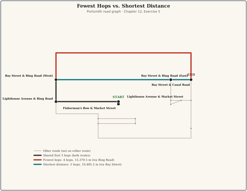
ORDER BY hops LIMIT 1 — plain breadth-first search —
optimizes for number of turns, not distance travelled,
and those are only the same question when every edge in the graph costs
roughly the same to traverse. They don’t, here, and a recursive CTE has
no built-in concept of “cost” unless a query explicitly asks it to
minimize one, the way 5.3’s ORDER BY total_m does instead
of 5.2’s ORDER BY hops. Real routing (turn-by-turn
navigation, Dijkstra’s algorithm, pgRouting) is built
entirely around taking that distinction seriously; this exercise is the
smallest possible version of the same lesson.
6.1 — A category tree built from real Chapter 1 data
SELECT c.name AS category, p.name AS parent
FROM categories c
JOIN categories p ON p.id = c.parent_id
WHERE c.name IN ('bakery', 'restaurant'); category | parent
------------+-----------------
restaurant | All Categories
bakery | restaurantcategories isn’t invented data — its two levels under
“All Categories” are exactly Chapter 1’s real category and
subcategory/cuisine values, pulled straight
out of businesses.details and organized into a tree.
“Bakery” is a real cuisine value on a real business (River Bend Bakery,
Chapter 1) three levels deep in this hierarchy.
6.2 — Walk up, then flatten into a breadcrumb
A faceted search UI wants “all ancestors of this leaf” to build a
breadcrumb trail — the exact same upward walk as Exercise 1, applied to
a different tree, finished off with string_agg:
WITH RECURSIVE ancestors AS (
SELECT id, name, parent_id, 0 AS depth
FROM categories
WHERE name = 'bakery'
UNION ALL
SELECT c.id, c.name, c.parent_id, ancestors.depth + 1
FROM categories c
JOIN ancestors ON c.id = ancestors.parent_id
)
SELECT string_agg(name, ' > ' ORDER BY depth DESC) AS breadcrumb
FROM ancestors; breadcrumb
---------------------------------------
All Categories > restaurant > bakeryORDER BY depth DESC inside string_agg puts
the root first and the leaf last — the walk itself discovers ancestors
leaf-to-root (depth increasing outward, exactly like
Exercise 1’s officer-to-Mayor chain), so displaying them root-to-leaf
means reversing that order at the very end, not changing how the
recursion runs. Nothing about this query knows or cares that the tree is
only three levels deep — the identical query against a ten-level
category tree would produce a ten-element breadcrumb without a single
line changing.
| Tool | What it does |
|---|---|
WITH RECURSIVE name AS (anchor UNION ALL recursive_term) |
Anchor runs once; the recursive term reruns against only the previous round’s new rows until a round adds nothing |
o.id = cte.manager_id |
Walk up a hierarchy — toward the root |
o.manager_id = cte.id |
Walk down a hierarchy — toward the leaves |
depth counter |
Increment it once per recursive round to know how deep any given row is |
path array + ORDER BY path |
Make a recursive CTE’s output print in proper depth-first tree order |
CYCLE col SET flag USING path |
Detect a repeated value instead of looping forever; flags the row where it happened |
WHERE NOT x = ANY(path) |
The hand-rolled version of cycle prevention, for graphs that need
per-branch path tracking CYCLE alone doesn’t give you |
SET statement_timeout |
Cheap insurance before running any recursive query over data you don’t control the integrity of |
BFS (ORDER BY hops) vs. shortest-distance
(ORDER BY total_m) |
Fewest steps and least total cost are different questions unless every edge costs the same |
string_agg(name, ' > ' ORDER BY depth DESC) |
Turn an ancestor walk into a breadcrumb, root first |
The key design insight from this chapter is that a
recursive CTE is just an ordinary query, run in a loop, over data that
happens to describe its own structure — the anchor decides where to
start, the join direction decides which way to walk, and everything past
that is the same SELECT you already know how to write.
Trees are the friendly case, where that loop is guaranteed to end
because nothing points back at itself. The moment real data — a bad
manager_id, a road network that loops — stops guaranteeing
that, the loop needs its own explicit exit condition, either
CYCLE’s built-in bookkeeping or a hand-rolled
path array doing the same job. Every exercise in this
chapter is one of exactly two ideas: which direction to walk, and how to
know when to stop.
Going further: Chapter 21’s placeholder chapter on PostgreSQL
19’s SQL/PGQ property graphs picks up directly from
Exercise 5 — the same road_segments graph, queried with
syntax purpose-built for path traversal instead of a hand-rolled
path array and a WHERE NOT ... ANY(...) guard.
Reading that chapter (once PostgreSQL 19 is out of beta and this book
can say something definite about it) right after this one, rather than
waiting for its place in the numbering, is a reasonable way to see the
same problem solved twice, eight chapters apart in the table of contents
but adjacent in what they’re actually about. Chapter 17’s foreign data
wrappers occasionally combine with recursive CTEs when a hierarchy spans
more than one database — the recursion itself doesn’t care where a row
physically lives, only that the self-referencing column resolves. And
pgRouting, mentioned briefly in Exercise 5, is the
production answer to “I need real shortest-path routing, not the
smallest example that demonstrates the idea” — turn restrictions,
one-way streets, and genuine Dijkstra/A implementations, all built
on top of the same PostGIS geometry this chapter’s road graph came
from.*
LISTEN/NOTIFY: Database-Native Pub/Sub“Polling asks ‘did anything happen yet?’ a thousand times a minute.
LISTENjust waits to be told.”
The obvious way to build a dashboard that reacts to database changes
is to ask, repeatedly:
SELECT * FROM jobs WHERE status = ..., once a second,
forever. It works, but every poll is a query the database has to answer
whether or not anything changed, and the dashboard is only ever as fresh
as its last poll — average half a polling interval stale, worst case a
whole interval. PostgreSQL has had a built-in alternative for longer
than most of its more famous features: LISTEN and
NOTIFY, a lightweight publish/subscribe system that ships
inside the database itself, no message broker required.
The shape of it is almost the whole idea: any session can run
LISTEN channel_name to subscribe to a named channel — just
a string, nothing has to be created or configured first. Any session —
or, more usefully, a trigger — can run NOTIFY channel_name
(optionally with a short text payload) to publish to it. Every session
currently listening on that channel gets the notification,
asynchronously, with no polling on anyone’s part.
Three things about when a notification actually arrives are easy to get wrong, so they’re worth stating plainly before Exercise 1 shows them happening:
NOTIFY inside a transaction
that later rolls back is as if it never ran — nothing is sent,
ever.psql) only check for and display it around the next command
they run — it doesn’t interrupt whatever the client is already
doing.NOTIFY calls on the same channel with the exact same
payload, inside the same transaction, are coalesced into a single
delivery.And one thing about what a notification isn’t: it has no
memory. NOTIFY doesn’t persist anything — if nobody is
listening on a channel the instant it fires, that notification is simply
gone. That’s why this chapter builds a second, very unglamorous thing
alongside the trigger: a plain table logging every notification ever
sent. NOTIFY says “wake up and go look”; the log table is
what a dashboard that just reconnected looks at to catch up on
whatever it missed while it was offline.
Portsmith’s permitting office wants a live status board for the job
queue Chapter 3 built — instead of a background process hammering
jobs on a timer, it should just be told the moment a
permit’s status changes.
| Object | Source | Purpose |
|---|---|---|
jobs |
Chapter 3 | The permit queue whose status changes this chapter reacts to |
notifications |
(built here) | Durable log of every notification sent — catch-up for a reconnecting dashboard |
notification_debounce |
(built here) | Last-notified timestamp per job, so Exercise 5 can suppress noisy bursts |
Nothing new needs seeding — this chapter is entirely about reacting to changes in data Chapter 3 already created.
By the end of this chapter you will be able to:
NOTIFY
whenever a row’s status changes.psycopg,
replacing a polling loop with a blocking wait for the next event.LISTEN/NOTIFY’s real throughput and
durability limits, and recognize the point past which a dedicated
message broker is the right call instead.Nothing to install. LISTEN and NOTIFY are
core SQL commands, part of PostgreSQL since long before this book’s
PostgreSQL 16 baseline — no extension, no configuration. This chapter’s
Python client (Exercise 3) reuses the psycopg driver
installed back in Chapter 1.
This chapter needs Chapter 3’s jobs table:
python data/ch03_seed.pySELECT COUNT(*) FROM jobs; count
-------
48
(1 row)(48, not 45 — Chapter 10’s PostgREST exercises filed three more permit applications through the API. If you’re at 45, that’s fine too; nothing in this chapter depends on the exact count.)
NOTIFY/LISTEN, Two Sessions1.1 — Subscribe in one session
Open two psql sessions side by side. In Session
A:
LISTEN portsmith_test;LISTENNothing else happens — LISTEN just registers this
session’s interest in the channel and returns immediately.
1.2 — Publish from the other
In Session B:
NOTIFY portsmith_test, 'hello from session B';NOTIFY1.3 — Back in Session A
Switch back to Session A. Nothing has appeared yet — run any statement to find out why:
SELECT 1; ?column?
----------
1
Asynchronous notification "portsmith_test" with payload "hello from
session B" received from server process with PID 2718842.The notification was sitting there the whole time, but
psql only surfaces it around the next command it sends —
exactly the second point from the Background section, now with a real
timestamp attached to it in the form of a PID you can watch change
between runs.
1.4 — A rolled-back NOTIFY never
arrives
With Session A still listening, run this in Session B:
BEGIN;
NOTIFY portsmith_test, 'should never arrive';
ROLLBACK;BEGIN
NOTIFY
ROLLBACKBack in Session A, run SELECT 1; again. Nothing prints —
no notification, no trace it was ever sent. NOTIFY inside a
transaction is exactly as durable as everything else in that
transaction: commit it or it didn’t happen.
1.5 — Identical notifications in one transaction collapse
BEGIN;
NOTIFY portsmith_test, 'dup';
NOTIFY portsmith_test, 'dup';
NOTIFY portsmith_test, 'dup';
COMMIT;Back in Session A:
SELECT 1;Asynchronous notification "portsmith_test" with payload "dup" received
from server process with PID 2721455.One delivery, not three. PostgreSQL deduplicates same-channel,
same-payload notifications within a single transaction before sending
anything — worth knowing before you assume a burst of identical
NOTIFYs inside one transaction will arrive as a burst on
the other end.
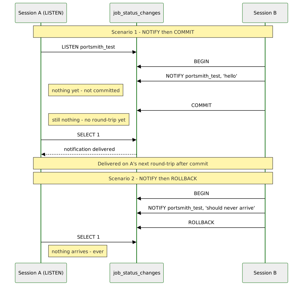
NOTIFYs on Status Change2.1 — The durable log
CREATE TABLE notifications (
id BIGSERIAL PRIMARY KEY,
channel TEXT NOT NULL,
payload JSONB NOT NULL,
created_at TIMESTAMPTZ NOT NULL DEFAULT clock_timestamp()
);2.2 — The trigger function
CREATE OR REPLACE FUNCTION notify_job_status_change() RETURNS TRIGGER AS $$
DECLARE
notice JSONB;
BEGIN
IF NEW.status IS DISTINCT FROM OLD.status THEN
notice := jsonb_build_object(
'job_id', NEW.id,
'job_type', NEW.job_type,
'old_status', OLD.status,
'new_status', NEW.status,
'changed_at', clock_timestamp()
);
INSERT INTO notifications (channel, payload) VALUES ('job_status_changes', notice);
PERFORM pg_notify('job_status_changes', notice::text);
END IF;
RETURN NEW;
END;
$$ LANGUAGE plpgsql;
CREATE TRIGGER trg_notify_job_status_change
AFTER UPDATE ON jobs
FOR EACH ROW
EXECUTE FUNCTION notify_job_status_change();IF NEW.status IS DISTINCT FROM OLD.status matters as
much as the NOTIFY itself — without it, this trigger fires
on any update to a job row, including the heartbeat timestamp
Chapter 3’s workers write every couple of seconds, flooding the channel
with “changes” where the status never actually moved.
pg_notify(channel, payload) is the function form of
NOTIFY — it takes both arguments as ordinary expressions,
which plain NOTIFY channel, 'literal' syntax can’t do, and
it’s what makes a computed channel name possible at all (Exercise 4
depends on exactly that).
2.3 — Trigger it
UPDATE jobs
SET status = 'in_progress', claimed_at = clock_timestamp(), claimed_by = 'worker-1'
WHERE id = (SELECT id FROM jobs WHERE status = 'queued' ORDER BY id LIMIT 1);A session already running LISTEN job_status_changes;
sees, on its next round-trip:
Asynchronous notification "job_status_changes" with payload
"{"job_id": 1, "job_type": "demolition_permit", "changed_at":
"2026-08-04T23:33:21.581832-04:00", "new_status": "in_progress",
"old_status": "queued"}" received from server process with PID 2734846.And the durable copy is sitting in the log table regardless of whether anyone was listening:
SELECT channel, payload, created_at FROM notifications; channel | payload | created_at
----------------------+----------------------------------------------------------------------------------+-------------------------------
job_status_changes | {"job_id": 1, "job_type": "demolition_permit", "old_status": "queued", ...} | 2026-08-04 23:33:21.582461-043.1 — A listener client
#!/usr/bin/env python3.12
# ch13_listen.py — Portsmith permit-status staff dashboard
import argparse
import json
import psycopg
def main() -> None:
parser = argparse.ArgumentParser(description=__doc__)
parser.add_argument("channels", nargs="*", default=["job_status_changes"])
parser.add_argument("--dsn", default="dbname=portsmith")
parser.add_argument("--timeout", type=float, default=None)
args = parser.parse_args()
with psycopg.connect(args.dsn, autocommit=True) as conn:
with conn.cursor() as cur:
for channel in args.channels:
cur.execute(f"LISTEN {channel};")
print(f"listening on {channel!r} …")
try:
for notice in conn.notifies(timeout=args.timeout):
job = json.loads(notice.payload)
print(
f"[{notice.channel}] job {job['job_id']} ({job['job_type']}): "
f"{job['old_status']} -> {job['new_status']}"
)
except KeyboardInterrupt:
print("\nstopped.")
if __name__ == "__main__":
main()autocommit=True matters here — LISTEN needs
to actually take effect immediately rather than sit inside an open
transaction waiting for a COMMIT that this script has no
reason to ever issue. conn.notifies(timeout=...) is a
generator: it blocks, doing nothing, until a notification arrives, then
yields it — no loop, no polling interval to tune, no SELECT
the database has to answer just to say “nothing’s changed.”
3.2 — Run it
python data/ch13_listen.pylistening on 'job_status_changes' …From a psql session, update another job’s status. The
moment that transaction commits:
[job_status_changes] job 2 (demolition_permit): queued -> completedNo delay, no polling — the script was simply asleep until PostgreSQL had something to tell it.
4.1 — One more pg_notify call
Public Works doesn’t want to see every business_license
update, and Permitting & Licensing doesn’t want to see every
demolition_permit update. Give each job type its own
channel, in addition to the all-activity one:
CREATE OR REPLACE FUNCTION notify_job_status_change() RETURNS TRIGGER AS $$
DECLARE
notice JSONB;
BEGIN
IF NEW.status IS DISTINCT FROM OLD.status THEN
notice := jsonb_build_object(
'job_id', NEW.id,
'job_type', NEW.job_type,
'old_status', OLD.status,
'new_status', NEW.status,
'changed_at', clock_timestamp()
);
INSERT INTO notifications (channel, payload) VALUES ('job_status_changes', notice);
PERFORM pg_notify('job_status_changes', notice::text);
PERFORM pg_notify('jobs_' || NEW.job_type, notice::text);
END IF;
RETURN NEW;
END;
$$ LANGUAGE plpgsql;'jobs_' || NEW.job_type builds the channel name from the
row being updated — jobs_business_license,
jobs_demolition_permit, and so on, five channels from one
trigger, none of them declared or created anywhere in advance. A channel
isn’t an object; it springs into existence the instant something
LISTENs or NOTIFYs it; and stops existing —
with nothing to clean up — the instant nothing is LISTENing
on it anymore.
CREATE OR REPLACE FUNCTION does exactly what it says —
replace, not patch or extend. This is now the third time this
chapter has redefined notify_job_status_change() in place
(Exercise 2’s version, this one, Exercise 5’s version still to come),
and there’s nothing tracking which version is currently live beyond
whatever the last CREATE OR REPLACE you ran actually said.
If you go back and re-run Exercise 2’s block for any reason —
double-checking something, copy-pasting the wrong snippet — you will
silently undo this one, with no error and no warning: the fan-out
channels just stop receiving anything, because the function that used to
pg_notify them no longer does. If a listener you expect to
see traffic suddenly goes quiet,
SELECT prosrc FROM pg_proc WHERE proname = 'notify_job_status_change'
is the fastest way to check which version is actually installed right
now.
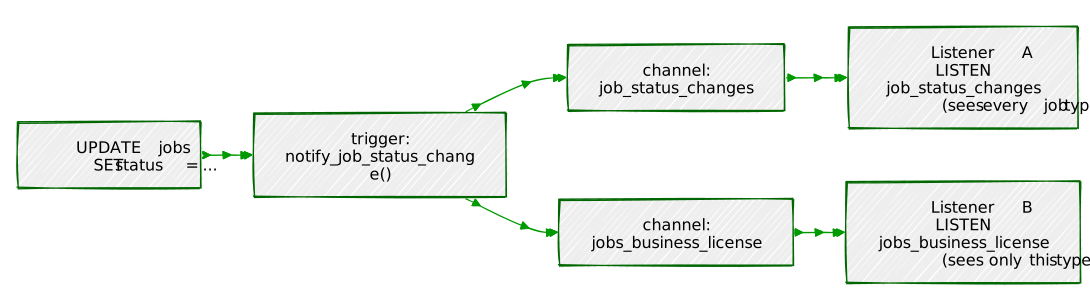
4.2 — Subscribe to just one
python data/ch13_listen.py jobs_business_licenselistening on 'jobs_business_license' …From a psql session, update a
building_permit job’s status, then a
business_license job’s status (building_permit
is used here, rather than the much smaller
demolition_permit pool, because it’s the largest job type —
15 permits — and least likely to have already run out of
queued rows from earlier testing; if a given
UPDATE reports 0 rows, that job type is simply
out of queued jobs right now, and any other job_type with
rows left makes the same point):
UPDATE jobs SET status = 'in_progress', claimed_at = clock_timestamp(), claimed_by = 'worker-1'
WHERE id = (SELECT id FROM jobs WHERE status = 'queued' AND job_type = 'building_permit' ORDER BY id LIMIT 1);
UPDATE jobs SET status = 'in_progress', claimed_at = clock_timestamp(), claimed_by = 'worker-1'
WHERE id = (SELECT id FROM jobs WHERE status = 'queued' AND job_type = 'business_license' ORDER BY id LIMIT 1);Only the second one shows up in the listener’s output:
[jobs_business_license] job 5 (business_license): queued -> in_progressThe building_permit change still fired — on
job_status_changes and on jobs_building_permit
— this listener simply never subscribed to either of those channels.
Fan-out costs nothing extra per additional channel; it’s just more
arguments to pg_notify.
5.1 — The problem
A job that flaps — fails, gets requeued, gets reclaimed, fails again, all within a second or two — fires a fresh notification on every single transition. A dashboard doesn’t need to render all of that; it needs to know where things ended up. Track, per job, when it was last actually notified about:
CREATE TABLE notification_debounce (
job_id BIGINT PRIMARY KEY,
last_notified_at TIMESTAMPTZ NOT NULL
);5.2 — Check it before sending
CREATE OR REPLACE FUNCTION notify_job_status_change() RETURNS TRIGGER AS $$
DECLARE
notice JSONB;
last_sent TIMESTAMPTZ;
BEGIN
IF NEW.status IS DISTINCT FROM OLD.status THEN
SELECT last_notified_at INTO last_sent
FROM notification_debounce WHERE job_id = NEW.id;
IF last_sent IS NOT NULL AND clock_timestamp() - last_sent < interval '1 second' THEN
RETURN NEW; -- too soon after the last one for this job — skip it
END IF;
notice := jsonb_build_object(
'job_id', NEW.id, 'job_type', NEW.job_type,
'old_status', OLD.status, 'new_status', NEW.status,
'changed_at', clock_timestamp()
);
INSERT INTO notifications (channel, payload) VALUES ('job_status_changes', notice);
PERFORM pg_notify('job_status_changes', notice::text);
PERFORM pg_notify('jobs_' || NEW.job_type, notice::text);
INSERT INTO notification_debounce (job_id, last_notified_at)
VALUES (NEW.id, clock_timestamp())
ON CONFLICT (job_id) DO UPDATE SET last_notified_at = EXCLUDED.last_notified_at;
END IF;
RETURN NEW;
END;
$$ LANGUAGE plpgsql;This is a leading-edge debounce: the first change in a burst fires immediately, and anything else for that same job within the next second is dropped — not delayed, not batched, just skipped. The status change itself still happens; only the notification about it is suppressed.
5.3 — Prove it
Four status changes on the same job, each about 200ms apart — well inside the 1-second window:
UPDATE jobs SET status = 'in_progress' WHERE id = 40;
UPDATE jobs SET status = 'failed' WHERE id = 40;
UPDATE jobs SET status = 'queued' WHERE id = 40;
UPDATE jobs SET status = 'in_progress' WHERE id = 40;A listener on job_status_changes sees exactly one of the
four:
[job_status_changes] job 40 (sign_permit): queued -> in_progressSELECT * FROM notification_debounce WHERE job_id = 40; job_id | last_notified_at
--------+-------------------------------
40 | 2026-08-04 23:59:04.475819-04Only one timestamp recorded — the second, third, and fourth updates
all checked it, found themselves inside the window, and returned without
touching it. Wait a full second and update the same job again: this time
it fires, because clock_timestamp() - last_sent has finally
crossed interval '1 second'.

6.1 — The payload ceiling is real, and it’s not quite 8000
SELECT pg_notify('sz', repeat('x', 7999)); -- succeeds
SELECT pg_notify('sz', repeat('x', 8000)); -- failsERROR: payload string too long7999 bytes is the actual limit, not the commonly quoted round 8000 — PostgreSQL reserves one byte for a terminator inside its fixed 8000-byte buffer. A JSON payload describing one row’s status change, the way this chapter’s trigger builds one, comes nowhere close; a payload trying to carry an entire row plus its full history would.
6.2 — Sending is not the bottleneck
DO $$
DECLARE
i INT;
start_time TIMESTAMPTZ := clock_timestamp();
BEGIN
FOR i IN 1..10000 LOOP
PERFORM pg_notify('throughput_test', 'msg ' || i);
END LOOP;
RAISE NOTICE 'Sent 10000 notifications in %', clock_timestamp() - start_time;
END $$;NOTICE: Sent 10000 notifications in 00:00:00.019504Ten thousand notifications, under twenty milliseconds, no listener even attached. The database can enqueue notifications far faster than any realistic client can usefully consume them — sending was never going to be where this architecture runs into trouble.
6.3 — Where it actually runs into trouble
The limits that matter are structural, not raw speed:
NOTIFY from every session, on every channel, goes into the
same queue. It isn’t partitioned by channel or topic the way a real
message broker’s queues are — a slow listener anywhere is a slow
listener for the whole mechanism.notifications table exists precisely because
LISTEN/NOTIFY has none on its own — a listener
down for five minutes misses everything that happened in those five
minutes, permanently, unless something else logged it.NOTIFY broadcasts to whoever happens to be listening right
now, once, with no concept of “did you actually process that.”NOTIFY traffic is a primary-only
affair — nothing to LISTEN for on a read replica will ever
arrive.None of that makes LISTEN/NOTIFY the wrong
tool — for exactly the job this chapter gave it, telling an
already-connected, already-trusted internal dashboard “something
changed, go look,” it’s close to free and requires nothing to operate.
The moment a requirement shows up that
LISTEN/NOTIFY structurally can’t satisfy —
guaranteed delivery across an outage, multiple independent consumer
groups, cross-database routing, back-pressure when a consumer falls
behind — that’s not a configuration problem to work around, it’s the
signal to bring in Kafka, RabbitMQ, or a similar dedicated broker
instead.
| Tool | What it does |
|---|---|
LISTEN channel |
Subscribe this session to a channel — created implicitly, no prior setup |
NOTIFY channel, 'payload' /
pg_notify(channel, payload) |
Publish to a channel; the function form allows computed channel names and expressions |
| Delivery timing | Only after the sending transaction commits; only noticed by a client on its next round-trip |
| Same-transaction dedup | Identical channel + payload, sent more than once in one transaction, delivers exactly once |
conn.notifies(timeout=...) (psycopg) |
A blocking generator — no polling loop, no interval to tune |
| Computed channel names | pg_notify('prefix_' \|\| value, ...) fans one trigger
out into many topic-scoped channels |
| A hand-built log table | The durability LISTEN/NOTIFY doesn’t
provide — what a reconnecting client catches up from |
| Leading-edge debounce (state table + timestamp check) | Fire the first event in a burst, suppress the rest within a window |
| 7999-byte payload ceiling | The real limit — 8000 minus a terminator byte |
| Structural limits: one shared queue, no persistence, no replay, primary-only | The reasons to graduate to a dedicated broker, not raw throughput |
The key design insight from this chapter is that
LISTEN/NOTIFY solves exactly one problem —
telling an already-connected session that something happened, right now,
cheaply — and solves nothing else on purpose. It has no memory, no
acknowledgment, no replay, no concept of a consumer that isn’t currently
connected. Every exercise past the first one was really about
compensating for that on purpose where it mattered (the log table for
durability, the debounce table for noise) and accepting it everywhere
else, because the alternative — a full message broker — is a lot of
operational weight to take on before you actually have a problem it
solves that this chapter’s five-line trigger doesn’t.
Going further: Chapter 14’s advisory locks are worth combining
with this chapter’s pattern the moment more than one process might react
to the same notification — nothing about
LISTEN/NOTIFY prevents two dashboards, or two
workers, from both trying to handle the same event. Chapter 18’s logical
replication is a different, heavier-weight answer to a similar-sounding
question (“tell me when a row changes”) — logical replication streams
the actual row changes themselves, durably, to another database, where
NOTIFY sends a fire-and-forget signal with an optional
short payload to whoever’s listening right now; reach for replication
when the requirement is “give me the data,” and
LISTEN/NOTIFY when it’s “just tell me to go
look.” And Chapter 19’s pg_cron pairs naturally with this
chapter’s notifications log table: a scheduled job that
sweeps for log rows newer than a dashboard’s last checkpoint is exactly
how that dashboard recovers from having been disconnected, the catch-up
path NOTIFY alone can never provide.
“Every lock in this book so far has been about a row. This one isn’t about any row at all.”
FOR UPDATE, row locks, SKIP LOCKED — every
locking mechanism this book has used up to now exists because two
transactions were reaching for the same data. But plenty of
real coordination problems have nothing to do with a specific row: “only
one process should run the nightly reconciliation job, whichever one
gets there first,” “elect a single leader among five identical workers,”
“make sure nobody else is already doing this whole category of work
right now.” There’s no row to lock for any of that — the thing you need
to coordinate around is an idea, not a record.
An advisory lock is PostgreSQL’s answer: a lock on a
plain integer you invent, with no connection to any table, row, or piece
of data whatsoever. You pick the number; PostgreSQL just remembers who’s
holding it and makes everyone else wait or ask. It’s called “advisory”
because nothing enforces that anyone respects it — unlike a row lock,
which UPDATE and DELETE are physically bound
by, an advisory lock only means anything to code that deliberately
checks it. That’s a feature, not a compromise: it’s a general-purpose
coordination primitive riding on a database your whole system probably
already talks to, instead of standing up ZooKeeper or etcd just to
answer “am I allowed to do this right now.”
Two choices you make every time you reach for one:
pg_advisory_lock() / pg_advisory_unlock() are
session-level — held until you explicitly unlock, or
your connection closes, whichever comes first.
pg_advisory_xact_lock() is
transaction-level — released automatically at
COMMIT or ROLLBACK, with no unlock function to
call and no way to release it early. Exercise 6 is entirely about a bug
that only one of these two is actually safe against.pg_advisory_lock() blocks until the lock is free.
pg_try_advisory_lock() returns immediately either way —
true if it got the lock, false if someone else
already holds it — which is what makes “is anyone else already doing
this?” a single non-blocking query instead of a hang.One more thing worth knowing before Exercise 1: like Chapter 13’s
NOTIFY, advisory locks are a primary-only affair. They live
in shared memory on whichever server you’re connected to, aren’t written
to WAL, and have no meaning at all on a streaming replica.
No new tables this chapter — it reuses Chapter 3’s jobs
queue and coordinates processes around it instead of adding
data.
| Object | Source | Purpose |
|---|---|---|
jobs |
Chapter 3 | The permit queue Exercise 4’s critical section guards |
data/ch14_leader_election.py |
(built here) | N simulated worker processes racing for one advisory lock |
By the end of this chapter you will be able to:
pg_try_advisory_lock() to ask “is anyone else
already doing this?” without waiting for an answer.pg_locks to see exactly which session holds which
advisory lock, and for how long.Nothing to install. Advisory locks are a core PostgreSQL feature — no extension, no configuration.
This chapter needs Chapter 3’s jobs table:
python data/ch03_seed.pySELECT COUNT(*) FROM jobs; count
-------
481.1 — Session A takes the lock
Open two psql sessions. In Session A,
pick an arbitrary key and lock it:
SELECT pg_advisory_lock(12345); pg_advisory_lock
------------------
(1 row)Returns immediately — nobody else holds 12345 yet.
12345 is not a row id, a job id, or a reference to
anything; it’s just a number this chapter picked, and every session that
agrees to use it for the same purpose is now coordinating through
it.
1.2 — Session B reaches for the same key
In Session B:
SELECT pg_advisory_lock(12345);Nothing comes back. The session just hangs — this is a real block, the same shape as waiting on a row lock, except there’s no row anywhere involved.
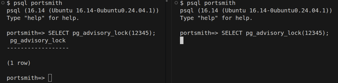
1.3 — Session A releases it
Back in Session A:
SELECT pg_advisory_unlock(12345); pg_advisory_unlock
--------------------
tThe instant this runs, Session B’s blocked query finally returns:
pg_advisory_lock
------------------
(1 row)Session B wasn’t retrying, polling, or checking back — it was
genuinely parked, waiting, and PostgreSQL woke it the moment the lock
freed up. (Session B is now holding 12345 itself; run
pg_advisory_unlock(12345) there before moving on.)
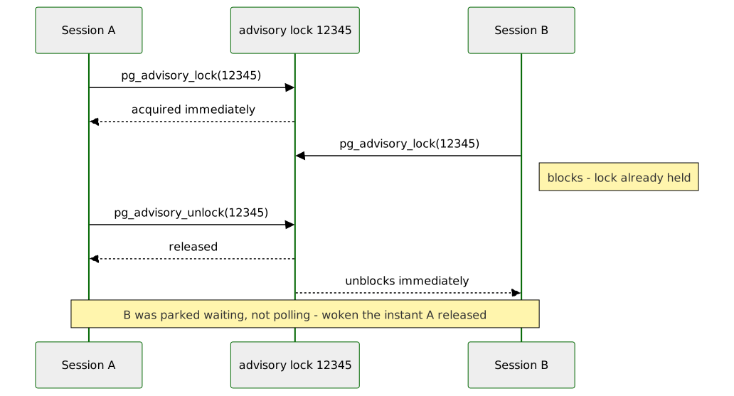
pg_try_advisory_lock(): Ask, Don’t Wait2.1 — The non-blocking version
With Session A still holding pg_advisory_lock(12345),
run this in Session B instead of the blocking form:
SELECT pg_try_advisory_lock(12345); pg_try_advisory_lock
-----------------------
f
(1 row)
Time: 0.029 msfalse, back in under a millisecond — no wait, no hang.
false means exactly one thing: someone currently
holds this key. true would mean the lock is now held by
you.
2.2 — Why this matters more than it looks
This single call is the entire mechanism behind “don’t start a second copy of this job if one’s already running.” A nightly batch job, a scheduled report, a background sweep — anything that must never run twice at once starts with exactly this check: try the lock, and if you don’t get it, exit immediately instead of doing the work. No polling table, no separate “is this running” flag to keep in sync with reality; the lock is the flag, and PostgreSQL can never let it lie about whether it’s held.
3.1 — Five workers, one leader
#!/usr/bin/env python3.12
# ch14_leader_election.py
import multiprocessing
import sys
import time
import psycopg
LEADER_LOCK_KEY = 99001
def worker(worker_id: int, dsn: str) -> None:
with psycopg.connect(dsn, autocommit=True) as conn:
with conn.cursor() as cur:
cur.execute("SELECT pg_try_advisory_lock(%s)", (LEADER_LOCK_KEY,))
(got_lock,) = cur.fetchone()
if got_lock:
print(f"[worker-{worker_id}] elected leader — starting work")
time.sleep(1.5)
print(f"[worker-{worker_id}] leader work done, releasing")
cur.execute("SELECT pg_advisory_unlock(%s)", (LEADER_LOCK_KEY,))
else:
print(f"[worker-{worker_id}] lost the race — standing by")
def main() -> None:
n_workers = int(sys.argv[1]) if len(sys.argv) > 1 else 5
dsn = sys.argv[2] if len(sys.argv) > 2 else "dbname=portsmith"
procs = [multiprocessing.Process(target=worker, args=(i, dsn)) for i in range(1, n_workers + 1)]
for p in procs:
p.start()
for p in procs:
p.join()
if __name__ == "__main__":
main()3.2 — Run it
python data/ch14_leader_election.py 5[worker-2] lost the race — standing by
[worker-3] lost the race — standing by
[worker-4] lost the race — standing by
[worker-5] lost the race — standing by
[worker-1] elected leader — starting work
[worker-1] leader work done, releasingEvery one of the five processes hits
pg_try_advisory_lock within microseconds of each other —
genuinely racing, not taking turns — and exactly one gets
true. Which worker wins is not deterministic; run it again
and a different number will win. What’s guaranteed isn’t who
becomes leader, only that there’s never more than one at a time. That
one guarantee is the entire value of leader election: five identical,
uncoordinated processes, and PostgreSQL — not any of them — is the
single source of truth for which one is in charge.
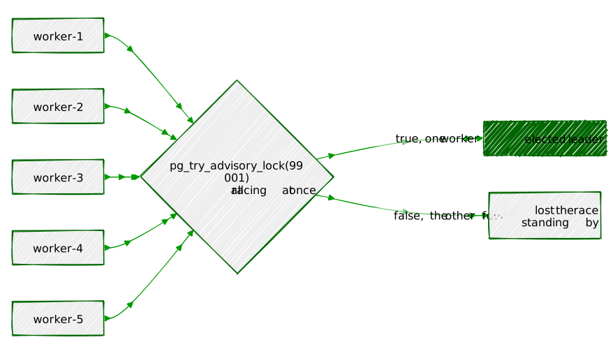
4.1 — A rule SKIP LOCKED can’t
express
Chapter 3’s FOR UPDATE SKIP LOCKED lets many workers
claim many different jobs rows at once, on purpose — that’s
the whole point of it. But suppose Portsmith has exactly one building
inspector, and city policy says only one demolition_permit
can be under active inspection at a time, no matter how many workers are
running or how many different demolition jobs are sitting in the queue.
Row locking can’t express “only one of this category,
regardless of which specific row” — that’s not a fact about any one row,
it’s a fact about all of them together. This is exactly what an advisory
lock, scoped to the job type rather than any job id, is for:
SELECT hashtext('demolition_permit'); hashtext
--------------
-1799557343hashtext() turns an arbitrary string into a
well-distributed integer — a convenient way to get a lock key out of a
category name without maintaining a lookup table mapping job types to
key numbers by hand.
4.2 — Wrap the claim in it
BEGIN;
SELECT pg_advisory_xact_lock(hashtext('demolition_permit'));
-- ... claim and begin working a demolition_permit job here ...
COMMIT;4.3 — Prove it serializes, even across different rows
The claim to check: two workers, claiming two different
demolition_permit jobs — nothing in common at the row level
— should still be forced to run one at a time, because the lock is
scoped to the category, not to either row. Open two psql
sessions again (same as Exercise 1) to watch it happen.
In Session A, run these three statements one at a
time, stopping after the third — do not run COMMIT yet:
BEGIN;
SELECT pg_advisory_xact_lock(hashtext('demolition_permit'));
SELECT 'worker A: claimed job 1, inspecting site...' AS status; pg_advisory_xact_lock
------------------------
(1 row)
status
---------------------------------------------
worker A: claimed job 1, inspecting site...
(1 row)Both statements return immediately — Session A now holds the lock,
and its transaction is deliberately left open (no COMMIT
yet) to simulate a worker still in the middle of an inspection.
Now switch to Session B and run this — a
different job, same demolition_permit
category:
BEGIN;
SELECT pg_advisory_xact_lock(hashtext('demolition_permit'));
SELECT 'worker B: got past the lock' AS status;
COMMIT;Session B hangs after BEGIN — the
pg_advisory_xact_lock call blocks, and the
status row never prints. Go back to Session
A and finally run:
COMMIT;The instant Session A’s transaction ends, Session B unblocks on its
own and finishes, printing worker B: got past the lock
followed by its own COMMIT. The lock released automatically
the moment Session A’s transaction closed — nothing had to explicitly
unlock it. Two entirely different job ids, no row either session touched
in common, and they were still fully serialized — because the thing
being protected was never a row to begin with.
pg_locks5.1 — The raw view
With a session holding pg_advisory_lock(12345) open
elsewhere:
SELECT locktype, ((classid::bigint << 32) | objid::bigint) AS lock_key,
mode, granted, pid
FROM pg_locks
WHERE locktype = 'advisory'; locktype | lock_key | mode | granted | pid
----------+----------+---------------+---------+---------
advisory | 12345 | ExclusiveLock | t | 2998844
(1 row)Advisory locks show up in pg_locks exactly like row and
table locks do — same catalog, same columns — except
locktype = 'advisory' and the “thing being locked” is just
a number PostgreSQL reconstructs from classid and
objid rather than a row identifier. That bit-shift
reassembles the single bigint key this chapter has been
passing to pg_advisory_lock() — session-level advisory
locks internally split a 64-bit key across those two 32-bit catalog
columns.
5.2 — A real diagnostic query
Raw pg_locks never tells you who or
why. Join it to pg_stat_activity for a query worth
keeping around:
SELECT l.pid,
((l.classid::bigint << 32) | l.objid::bigint) AS lock_key,
l.mode, l.granted,
a.usename, a.application_name,
now() - a.state_change AS held_for,
a.query AS last_query
FROM pg_locks l
JOIN pg_stat_activity a ON a.pid = l.pid
WHERE l.locktype = 'advisory'; pid | lock_key | mode | granted | usename | application_name | held_for | last_query
---------+----------+---------------+---------+---------+-------------------+-----------------+----------------------------------
2999823 | 12345 | ExclusiveLock | t | chris | psql | 00:00:00.53227 | SELECT pg_advisory_lock(12345);
(1 row)held_for is the question that actually matters in
production: a lock held for 30 milliseconds is a Tuesday; a lock held
for 6 hours because some process crashed without releasing it is an
incident. This query is exactly what you’d point a monitoring check
at.
6.1 — Session locks assume “session” means what you think it means
pg_advisory_lock()’s session-level lifetime is a
promise: the lock lives exactly as long as your database connection
does. That promise quietly breaks the moment a connection pool sits
between your application and PostgreSQL, because a pooled connection’s
physical lifetime and any one request’s logical
lifetime are no longer the same thing. Simulate it directly — one
physical connection, reused across two completely unrelated pieces of
work, the way a pool would hand it out twice:
import psycopg
POOL_KEY = 55001
pooled_conn = psycopg.connect("dbname=portsmith", autocommit=True)
# --- "Request 1": nightly reconciliation job start ---
with pooled_conn.cursor() as cur:
cur.execute("SELECT pg_advisory_lock(%s)", (POOL_KEY,))
print("[request 1] acquired session lock", POOL_KEY)
# BUG: request 1 finishes (or crashes) without calling pg_advisory_unlock.
print("[request 1] done — connection returned to pool (lock still held!)")
# --- "Request 2": unrelated request, later, same physical connection ---
with pooled_conn.cursor() as cur:
cur.execute("SELECT pg_try_advisory_lock(%s)", (POOL_KEY,))
(got_lock,) = cur.fetchone()
print(f"[request 2] pg_try_advisory_lock({POOL_KEY}) -> {got_lock}")[request 1] acquired session lock 55001
[request 1] done — connection returned to pool (lock still held!)
[request 2] pg_try_advisory_lock(55001) -> True (same physical session as request 1!)Request 2 gets True and has every reason to believe it’s
the exclusive holder of key 55001 — leader, singleton,
whatever that key was supposed to mean — and it’s completely wrong.
PostgreSQL sees one session that already held the lock asking for it
again, which is trivially true by definition; it has no way
to know “request 1” and “request 2” were ever meant to be different
things. This is the bug the guide warns about, and it is exactly as
dangerous as it sounds: two unrelated requests, coordinating through a
lock that was never really shared between them, both convinced they’re
safe.
6.2 — The fix: use the lock type that can’t leak
import psycopg
POOL_KEY = 55002
pooled_conn = psycopg.connect("dbname=portsmith") # autocommit off
# --- "Request 1", transaction-scoped this time ---
with pooled_conn.cursor() as cur:
cur.execute("SELECT pg_advisory_xact_lock(%s)", (POOL_KEY,))
print("[request 1] acquired xact lock", POOL_KEY)
pooled_conn.commit() # released here, no matter what request 1 does or forgets
print("[request 1] committed — lock released automatically")
# --- "Request 2", same pooled connection ---
with pooled_conn.cursor() as cur:
cur.execute("SELECT pg_try_advisory_lock(%s)", (POOL_KEY,))
(got_lock,) = cur.fetchone()
print(f"[request 2] pg_try_advisory_lock({POOL_KEY}) -> {got_lock} (correctly free)")[request 1] acquired xact lock 55002
[request 1] committed — lock released automatically
[request 2] pg_try_advisory_lock(55002) -> True (correctly free)Same reused connection, same shape of bug waiting to happen — but
this time request 2’s true is
correct, because pg_advisory_xact_lock physically
cannot survive past COMMIT. There’s no unlock call to
forget, no code path where an exception skips the cleanup, because
there’s no cleanup step at all: the transaction boundary is the
release. The rule this exercise earns: reach for
pg_advisory_xact_lock(), not
pg_advisory_lock(), for anything that might ever run behind
a connection pool — which, in most modern application deployments, is
close to everything.
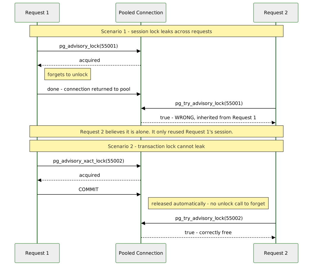
| Tool | What it does |
|---|---|
pg_advisory_lock(key) /
pg_advisory_unlock(key) |
Session-level lock — held until explicitly released or the connection closes |
pg_advisory_xact_lock(key) |
Transaction-level lock — released automatically at
COMMIT/ROLLBACK, no unlock function
exists |
pg_try_advisory_lock(key) |
Non-blocking — true/false immediately
instead of waiting |
hashtext('a category name') |
Turn an arbitrary string into a lock key without a lookup table |
| Leader election pattern | N processes pg_try_advisory_lock the same key; exactly
one gets true |
| Critical-section pattern | pg_advisory_xact_lock around a category-wide rule row
locking can’t express |
pg_locks WHERE locktype = 'advisory' |
See every held advisory lock, joined to
pg_stat_activity for who/how long |
| Connection-pool pitfall | A session lock can leak across unrelated pooled requests; a transaction lock structurally cannot |
The key design insight from this chapter is that
advisory locks trade specificity for reach: a row lock only ever means
“this row,” but an advisory lock can mean anything at all, because the
number means whatever your application agrees it means. That flexibility
is also the whole risk — nothing stops two unrelated parts of a codebase
from picking the same integer by accident, and nothing stops a
session-level lock from outliving the logical operation it was meant to
protect the instant a connection pool gets involved. Every exercise past
the first two was really about earning back the specificity a row lock
gets for free: naming a category clearly (hashtext),
choosing a lifetime that matches the actual unit of work (transaction,
not session), and knowing how to ask PostgreSQL, out loud, exactly who’s
holding what.
Going further: Chapter 19’s pg_cron is where the
singleton-job pattern from Exercise 2 stops being a hypothetical — a
scheduled job that might occasionally overlap its own next run is the
textbook case for wrapping the job body in
pg_try_advisory_lock and exiting quietly if it doesn’t get
it. Chapter 13’s NOTIFY and this chapter’s advisory locks
share the same primary-only limitation, and for the same underlying
reason: both live in server-local memory rather than WAL, so neither one
is a tool for coordinating across a primary and its replicas — that
requires the data itself to be replicated, which is Chapter 18’s
subject. And it’s worth holding onto the contrast with Chapter 3
explicitly: FOR UPDATE SKIP LOCKED coordinates access to
rows that exist; advisory locks coordinate processes,
around ideas that were never going to have a row of their own no matter
how the schema was designed.
“A
CHECKconstraint says ‘reject this if it’s wrong.’ A type says ‘wrong isn’t a value this column can even hold.’”
Every table in this book so far has leaned on CHECK
constraints and plain base types — TEXT,
INTEGER, JSONB — to keep bad data out. That
works, but it puts the rule next to the column rather than
in it: jobs.status has always been a
TEXT column that happens to carry a
CHECK (status IN (...)) alongside it, and nothing about the
column’s own type tells you that. PostgreSQL’s type system lets you go
one level deeper and make the rule part of the type itself.
Three tools, three different jobs:
CREATE TYPE ... AS ENUM (...))
replace “a TEXT column with a CHECK list” with
a real type that can only hold one of a fixed set of labels.
The database rejects anything else the moment you try to store it — not
as a constraint violation, but as a type error, the same category of
rejection as trying to put text in an integer column.CREATE DOMAIN ... AS base_type CHECK (...)) attach a
constraint to an existing type and give the result a name — a
positive_integer is still an INTEGER
underneath, but any column declared with that domain inherits the check
automatically, once, instead of you retyping the same CHECK
clause on every column that needs it.CREATE TYPE ... AS (...)) bundle several named fields into
one type, the way a table’s row type already works, except you can use
it as the type of a single column — a contact_info
value is one column that internally holds a phone number, a postcode,
and a preferred contact method together.All three live in the database’s own catalog, which means every tool
that talks to PostgreSQL can discover them — a psycopg client, a
PostgREST endpoint, even psql’s own \d output
— without you writing a line of validation logic anywhere outside the
schema. Exercise 6 is where that pays off directly.

This chapter adds typed columns to three tables already in the book, rather than any new ones:
| Table | New column | Type |
|---|---|---|
jobs (Ch3) |
status (converted in place) |
job_status enum |
businesses (Ch1) |
employee_count |
positive_integer domain |
residents (Ch5) |
contact |
contact_info composite (embeds a
uk_postcode domain) |
residents (Ch5) |
email |
email_address domain |
jobs.status already existed as TEXT with a
CHECK constraint — Exercise 1 converts it to a real enum in
place, which turns out to be more interesting than it sounds, because
Chapter 10’s api.jobs view is still sitting on top of
it.
By the end of this chapter you will be able to:
CHECK-constrained TEXT
column into a proper ENUM, and know every kind of object
that can block that conversion before it actually works.CHECK.Nothing to install. CREATE TYPE,
CREATE DOMAIN, and enums are all core SQL, no extension
required. Exercise 6 reuses psycopg (Chapter 1) and,
optionally, PostgREST (Chapter 10) if you still have it configured.
This chapter needs Chapters 1, 3, and 5’s data:
python data/ch01_seed.py # businesses
python data/ch03_seed.py # jobs
python data/ch05_seed.py # residentsSELECT 'businesses' AS table, COUNT(*) FROM businesses
UNION ALL SELECT 'jobs', COUNT(*) FROM jobs
UNION ALL SELECT 'residents', COUNT(*) FROM residents; table | count
---------------+-------
businesses | 48
jobs | 48
residents | 58TEXT + CHECK Into a Real Enum1.1 — Define the type
CREATE TYPE job_status AS ENUM ('queued', 'in_progress', 'completed', 'failed');This creates the type — it doesn’t touch jobs yet.
jobs.status is still TEXT, still governed by
the original CHECK constraint from Chapter 3.
1.2 — Three things that block the conversion, in the order you’ll hit them
The obvious next move —
ALTER TABLE jobs ALTER COLUMN status TYPE job_status USING status::job_status;
— fails, and it fails for three separate reasons if you fix them one at
a time instead of all at once. Each is worth seeing for real, because
each is a genuinely common shape of dependency in any schema that’s been
alive for more than one chapter:
Blocker 1 — the column’s own default:
ERROR: default for column "status" cannot be cast automatically to type job_statusstatus DEFAULT 'queued' was set while the column was
TEXT; the default expression has to be dropped before the
column type can change, and re-added afterward.
Blocker 2 — a dependent view:
ERROR: cannot alter type of a column used by a view or rule
DETAIL: rule _RETURN on view api.jobs depends on column "status"Chapter 10’s api.jobs view selects status
directly. PostgreSQL won’t silently change a column’s type out from
under a view built on top of it — the view has to be dropped and
recreated around the change. This is exactly the kind of cross-chapter
dependency a real production schema accumulates constantly, and exactly
why this exercise is worth doing on the actual multi-chapter database
instead of a clean scratch table.
Blocker 3 — a dependent partial index:
ERROR: operator does not exist: job_status = text
HINT: No operator matches the given name and argument types.idx_jobs_claim_order (Chapter 3) is a partial index with
WHERE status = 'queued' baked into it. Once
status is no longer TEXT, PostgreSQL has to
rebuild that stored predicate — and a bare
job_status = text comparison doesn’t exist as an operator;
enums don’t implicitly compare against a different type the way a
literal implicitly resolves against a column of a known type. This index
has to be dropped and rebuilt too.

1.3 — The full sequence, correctly ordered, in one transaction
Run this as postgres, not your regular login role —
sudo -u postgres psql portsmith. api.jobs is
owned by postgres (it was created from that same role back
in Chapter 10, Exercise 1.1), and a normal login role typically has no
USAGE on the api schema at all, let alone
ownership of the view sitting in it. Trying to run this as your own role
fails immediately with permission denied for schema api
before it ever gets near the actual type conversion:
BEGIN;
DROP VIEW IF EXISTS api.jobs;
DROP INDEX IF EXISTS idx_jobs_claim_order;
ALTER TABLE jobs ALTER COLUMN status DROP DEFAULT;
ALTER TABLE jobs DROP CONSTRAINT IF EXISTS jobs_status_check;
ALTER TABLE jobs ALTER COLUMN status TYPE job_status USING status::job_status;
ALTER TABLE jobs ALTER COLUMN status SET DEFAULT 'queued'::job_status;
CREATE INDEX IF NOT EXISTS idx_jobs_claim_order
ON jobs (priority, created_at, id)
WHERE status = 'queued';
CREATE VIEW api.jobs AS
SELECT id, job_type, payload, priority, status, created_at
FROM jobs;
GRANT SELECT ON api.jobs TO web_anon;
GRANT INSERT (job_type, payload, priority) ON api.jobs TO web_anon;
COMMIT;Wrapping the whole thing in BEGIN/COMMIT
matters here specifically because psql’s non-interactive
-f mode does not wrap a script in one implicit
transaction the way a -c "stmt1; stmt2;" invocation does —
without the explicit BEGIN, a failure partway through a
script like this one leaves the schema in whatever half-converted state
the successful statements got it to, which is exactly what happened
during this chapter’s own testing before the transaction wrapper was
added.
The IF EXISTS/IF NOT EXISTS on every
DROP/CREATE above earn their keep for the same
reason: because the whole block is one transaction, any single failure
aborts everything in it, including statements that already succeeded —
so if this script is ever run a second time (after an earlier run
partially failed, or simply to double-check the result), the objects
from a previous successful run are still sitting there. Without
IF EXISTS, a re-run’s
DROP CONSTRAINT jobs_status_check would error with
“constraint … does not exist” the moment status is already
a job_status, aborting the whole transaction over nothing
actually wrong. With it, this script is safe to run again at any point —
fully unconverted, partially converted, or already done — and either
converges to the same end state or changes nothing at all.
1.4 — Confirm it, and confirm the rejection
\d jobs status | job_status | | not null | 'queued'::job_status
...
Indexes:
"idx_jobs_claim_order" btree (priority, created_at, id) WHERE status = 'queued'::job_statusUPDATE jobs SET status = 'archived_forever' WHERE id = 1;ERROR: invalid input value for enum job_status: "archived_forever"(Deliberately not 'cancelled' here — Exercise 2 is about
to make that one a real value, and if you’re re-running this exercise on
a database that’s already been through Exercise 2,
'cancelled' would no longer be rejected.
'archived_forever' is never added anywhere in this chapter,
so this check stays valid no matter what order you run things in or how
many times you re-run it.)
Compare this to Chapter 3’s original CHECK violation
message — same outcome, a rejected write, but a completely different
category of error. 'archived_forever' isn’t
disallowed, from PostgreSQL’s point of view; it simply isn’t a
job_status at all, the same way 'abc' isn’t an
INTEGER.
2.1 — Add a value
ALTER TYPE job_status ADD VALUE 'cancelled';
SELECT enum_range(NULL::job_status); enum_range
---------------------------------------------------
{queued,in_progress,completed,failed,cancelled}New values are appended at the end by default.
enum_range returns every label in the type’s actual sort
order — enums order by declaration position, not
alphabetically, which is why 'cancelled' sorts after
'failed' here despite the alphabet disagreeing.
2.2 — Control exactly where it lands
ALTER TYPE job_status ADD VALUE 'on_hold' BEFORE 'in_progress';
SELECT enum_range(NULL::job_status); enum_range
---------------------------------------------------------
{queued,on_hold,in_progress,completed,failed,cancelled}BEFORE/AFTER exist precisely because
append-only ordering isn’t always what you want — 'on_hold'
belongs conceptually between queued and
in_progress, and now it sorts there too, which matters
anywhere this column gets used in an ORDER BY.
2.3 — The rule that catches almost everyone once
BEGIN;
ALTER TYPE job_status ADD VALUE 'archived';
UPDATE jobs SET status = 'archived' WHERE id = 1;
COMMIT;ERROR: unsafe use of new value "archived" of enum type job_status
HINT: New enum values must be committed before they can be used.ADD VALUE is allowed inside a transaction block — that
restriction was lifted back in PostgreSQL 12 — but the new label still
can’t be used until the transaction that added it actually
commits. PostgreSQL can’t yet guarantee the value will still exist if
this transaction rolls back, so it refuses to let anything reference it
in the meantime. (This transaction did roll back here, which is exactly
why 'archived' doesn’t appear in 2.2’s output above — the
ADD VALUE itself is fully transactional too.) Add the value
and use it in two separate transactions, and this is a non-issue.
positive_integer Domain3.1 — Define it once, use it anywhere
CREATE DOMAIN positive_integer AS INTEGER CHECK (VALUE > 0);
ALTER TABLE businesses ADD COLUMN employee_count positive_integer;VALUE inside a domain’s CHECK refers to
whatever’s being validated — the same role NEW.column plays
in a trigger, just scoped to a single value instead of a whole row.
3.2 — It enforces itself, everywhere, immediately
UPDATE businesses SET employee_count = 12 WHERE name = 'The Gilded Clam';UPDATE 1UPDATE businesses SET employee_count = -5 WHERE name = 'Anchor & Oar Tavern';ERROR: value for domain positive_integer violates check constraint "positive_integer_check"UPDATE businesses SET employee_count = 0 WHERE name = 'Anchor & Oar Tavern';ERROR: value for domain positive_integer violates check constraint "positive_integer_check"Zero fails too — > 0, not >= 0, meant
exactly what it said. Every future column ever declared
positive_integer gets this exact rule for free, with no
CHECK clause to remember to copy.
contact_info Composite Type4.1 — A domain nested inside a composite type
Portsmith’s real-world namesake, Portsmouth, England, has postcodes starting with “PO” — worth getting right rather than reaching for a generic example:
CREATE DOMAIN uk_postcode AS TEXT
CHECK (VALUE ~ '^[A-Z]{1,2}[0-9][A-Z0-9]? [0-9][A-Z]{2}$');
CREATE TYPE contact_info AS (
phone TEXT,
postcode uk_postcode,
preferred_contact TEXT
);
ALTER TABLE residents ADD COLUMN contact contact_info;A composite type’s fields aren’t limited to base types —
postcode here is a full domain, constraint included, nested
one level inside another type. Validation composes the same way the
types do.
4.2 — Store and query it
UPDATE residents
SET contact = ROW('023 9281 4477', 'PO1 3AX', 'phone')::contact_info
WHERE full_name = 'Adrian Foscolo';SELECT full_name, (contact).phone, (contact).postcode
FROM residents
WHERE full_name = 'Adrian Foscolo'; full_name | phone | postcode
------------------+---------------+----------
Adrian Foscolo | 023 9281 4477 | PO1 3AX(contact).phone — the parentheses are required; without
them, contact.phone parses as “column phone of
table contact,” not “field phone of column
contact.” One column, \d residents shows one
contact_info entry, but it carries three named,
individually queryable fields.
4.3 — The nested domain still enforces itself
UPDATE residents
SET contact = ROW('023 9281 0000', 'NOTVALID', 'email')::contact_info
WHERE full_name = 'Marisol Quintero';ERROR: value for domain uk_postcode violates check constraint "uk_postcode_check"The CHECK fires from two levels down — PostgreSQL
validates every domain-typed field of a composite value the same way it
would validate a plain column, whether or not that field happens to be
buried inside something else on its way into the table.
5.1 — A dedicated, standalone domain
CREATE DOMAIN email_address AS TEXT
CHECK (VALUE ~ '^[A-Za-z0-9._%+-]+@[A-Za-z0-9.-]+\.[A-Za-z]{2,}$');
ALTER TABLE residents ADD COLUMN email email_address;5.2 — Two different ways to fail
UPDATE residents SET email = 'adrian.foscolo@example.com' WHERE full_name = 'Adrian Foscolo';UPDATE 1UPDATE residents SET email = 'not-an-email' WHERE full_name = 'Marisol Quintero';ERROR: value for domain email_address violates check constraint "email_address_check"UPDATE residents SET email = 'someone@localhost' WHERE full_name = 'Marisol Quintero';ERROR: value for domain email_address violates check constraint "email_address_check"'someone@localhost' is a technically-valid email address
by the actual internet standard — real mail servers accept it — and this
regex still rejects it, because it has no .-separated
top-level domain. Every regex-based domain like this one is a
deliberate, imperfect trade: strict enough to catch obvious garbage,
permissive enough not to reject real addresses your business actually
needs, and never a substitute for verifying an address by actually
sending mail to it.
6.1 — psycopg, by default
import psycopg
with psycopg.connect("dbname=portsmith") as conn:
with conn.cursor() as cur:
cur.execute("SELECT id, status FROM jobs WHERE id = 1;")
row = cur.fetchone()
print(f"value: {row[1]!r}")
print(f"python type: {type(row[1])}")value: 'in_progress'
python type: <class 'str'>No configuration, no registration — an enum column just arrives as a
plain Python string, because PostgreSQL’s own wire protocol already
tells the driver “this value is text-shaped,” and psycopg
doesn’t need to know anything about job_status specifically
to hand it back correctly.
6.2 — psycopg, fully reflected as a real Python
enum
import psycopg
from psycopg.types.enum import register_enum, EnumInfo
with psycopg.connect("dbname=portsmith") as conn:
info = EnumInfo.fetch(conn, "job_status")
register_enum(info, conn)
print("labels from the database:", info.labels)
with conn.cursor() as cur:
cur.execute("SELECT id, status FROM jobs WHERE id = 1;")
row = cur.fetchone()
print(f"value: {row[1]!r}")
print(f"python type: {type(row[1])}")labels from the database: ['queued', 'on_hold', 'in_progress', 'completed', 'failed', 'cancelled']
value: <Job_Status.in_progress: 3>
python type: <enum 'Job_Status'>EnumInfo.fetch() reads the live set of labels
straight out of pg_enum — all six, including
on_hold and cancelled from Exercise 2 — and
register_enum() builds and wires up a real Python
enum.Enum class from them, on the spot. Change the
database’s enum next month and this code doesn’t change at all; it
reflects whatever the type currently contains.
6.3 — PostgREST’s OpenAPI document
With PostgREST running against this database (Chapter 10’s setup):
curl -s http://localhost:3000/ | jq '.definitions.jobs.properties.status'{
"enum": ["queued", "on_hold", "in_progress", "completed", "failed", "cancelled"],
"format": "public.job_status",
"type": "string"
}The exact same six labels, discovered the exact same way — by
introspecting job_status directly — and published
automatically in the API’s own schema document. No route was written to
expose this list anywhere; it’s a side effect of the column’s type being
what it is.
6.4 — And the API enforces it too, for free
curl -s "http://localhost:3000/jobs?status=eq.bogus"{"code":"22P02","details":null,"hint":null,"message":"invalid input value for enum job_status: \"bogus\""}curl -s -o /dev/null -w "%{http_code}\n" "http://localhost:3000/jobs?status=eq.bogus"400The exact same error PostgreSQL raised back in Exercise 1.4, now
arriving as a 400 over HTTP with PostgreSQL’s own error
code and message intact. PostgREST didn’t validate this value against a
list it maintains — it never has to. The type validated it, at the one
place that was always going to be authoritative regardless of which
client asked.
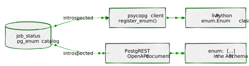
| Tool | What it does |
|---|---|
CREATE TYPE name AS ENUM (...) |
A type that can only hold one of a fixed set of labels |
ALTER TABLE ... ALTER COLUMN ... TYPE enum USING col::enum |
Convert an existing column — after clearing its default and any dependent views/indexes |
ALTER TYPE ... ADD VALUE [BEFORE\|AFTER 'x'] |
Add a label; position controls sort order, not just membership |
| New enum values in a transaction | Addable, but unusable until that transaction commits |
CREATE DOMAIN name AS base_type CHECK (VALUE ...) |
A named, reusable constraint on top of an existing type |
CREATE TYPE name AS (field type, ...) |
A composite type — several named fields as one column |
(composite_col).field |
Access one field of a composite column — parentheses required |
| A domain nested inside a composite field | Still fully enforced, at whatever depth it’s used |
EnumInfo.fetch() + register_enum()
(psycopg) |
Build a live Python Enum class from a database enum’s
current labels |
PostgREST’s / OpenAPI document |
Lists a column’s enum values automatically, from the type, with no route written for it |
The key design insight from this chapter is where
the rule actually lives. A CHECK constraint and a custom
type can enforce the identical rule — Chapter 3’s original
status IN (...) and this chapter’s job_status
enum reject exactly the same bad values — but only one of them is a fact
every tool touching the database can discover on its own, without being
told. psycopg didn’t need to be taught what
job_status allows; PostgREST didn’t need a hand-written
validator for it either. Both found out by asking PostgreSQL, because
the rule was never bolted onto the column from outside — it was what the
column’s type actually was.
Going further: Chapter 16’s generated columns are this chapter’s
natural next step — where a domain or enum constrains what a column can
hold, a generated column controls what a column is,
computed automatically from the rest of the row. The
positive_integer and email_address domains
built here are deliberately simple; production schemas often layer
several domains and composite types together the way
contact_info nested uk_postcode in Exercise 4,
one constraint at a time, until the type system is carrying most of what
used to live in application-layer validation code. And Exercise 1’s
dependency chain — a default, a view, a partial index, all blocking one
column’s type change — is worth remembering the next time any column
with a few chapters of history behind it needs to change shape:
\d on the table first, always, before the
ALTER.
“A trigger is a promise that someone wrote the sync logic correctly. A generated column is a fact that there was never anything else it could have contained.”
Chapter 4’s city_documents.search_vector and Chapter
13’s notify_job_status_change() both solve the same
underlying problem — “keep a derived value in sync with the columns it’s
computed from” — the same way: a trigger, hand-written, that fires on
INSERT/UPDATE and recomputes the value. It
works, but it works because someone wrote it correctly, remembered to
fire it on the right columns, and never introduced a code path that
updates the base columns without also firing the trigger. A
generated column removes all three of those “someone
remembered to” risks by making the derivation part of the column’s own
definition:
column_name type GENERATED ALWAYS AS (expression) STOREDSTORED isn’t optional decoration — as of the PostgreSQL
version this book targets, STORED is the only kind
of generated column PostgreSQL supports. The expression is computed
once, at write time, and the result is physically written to disk right
alongside every other column, not recomputed on every read. There’s no
trigger to find, no function to audit, no risk of an UPDATE
statement somewhere that touches the base columns without going through
the trigger — because GENERATED ALWAYS means exactly that.
PostgreSQL enforces it directly: Exercise 4 tries to write to one on
purpose, just to watch it refuse.
The one requirement that makes this possible, and the thing to hold onto before Exercise 1’s first real surprise: the expression must be immutable — given the same input row, it must always produce the same output, forever, with no dependency on anything outside that row. That sounds like a formality until it collides with something this book has run into more than once already.
| Table | Column | Computed from |
|---|---|---|
sensor_readings (Ch8) |
reading_date |
recorded_at, date portion only |
businesses (Ch1) |
search_vector |
name + several details JSONB fields |
city_documents (Ch4) |
search_vector |
title + body — replaces a hand-written
trigger |
residents (Ch15) |
phone_digits |
(contact).phone, digits only |
Every one of these already has real data behind it from earlier chapters — this chapter is entirely about adding computed columns to tables that already exist, not seeding anything new.
By the end of this chapter you will be able to:
tsvector column with a generated column that does the same
job declaratively.Nothing to install. Generated columns are core SQL, available since PostgreSQL 12.
This chapter needs Chapters 1, 4, 5, 8, and 15’s data already in place:
python data/ch01_seed.py # businesses
python data/ch04_seed.py # city_documents
python data/ch05_seed.py # residents
python data/ch08_seed.py # sensors; then Chapter 8's own exercises to build sensor_readingsChapter 15’s contact_info composite type and
residents.contact column need to exist too — see that
chapter if you haven’t run it yet.
SELECT 'sensor_readings' AS table, COUNT(*) FROM sensor_readings
UNION ALL SELECT 'businesses', COUNT(*) FROM businesses
UNION ALL SELECT 'city_documents', COUNT(*) FROM city_documents
UNION ALL SELECT 'residents', COUNT(*) FROM residents; table | count
-------------------+---------
sensor_readings | 9648001
businesses | 48
city_documents | 30
residents | 58(9,648,001, not 9,648,000 — Chapter 9, Exercise 5.3’s late-arriving traffic reading is still in there. If you’re at an even 9,648,000, that’s fine too; nothing here depends on the exact count.)
1.1 — The obvious expression fails
ALTER TABLE sensor_readings
ADD COLUMN reading_date DATE GENERATED ALWAYS AS (recorded_at::date) STORED;ERROR: generation expression is not immutablerecorded_at is TIMESTAMPTZ — an absolute
instant, not a calendar date. Casting it to DATE requires
picking a timezone to interpret that instant in, and a bare
::date cast uses whatever the current session’s
timezone setting happens to be. Two sessions with different
timezone settings would compute two different dates from the identical
recorded_at value — which is exactly what “not immutable”
means: PostgreSQL refuses to store a value that isn’t guaranteed to be
the same answer forever, computed from the row alone. This is the same
class of bug Chapters 8, 9, and 11 all had to work around by hand with
SET timezone = 'UTC'; at the top of every session — except
here, PostgreSQL catches it at CREATE time instead of
letting it silently produce different numbers depending on who’s
connected.
1.2 — Pin the timezone inside the expression itself
ALTER TABLE sensor_readings
ADD COLUMN reading_date DATE
GENERATED ALWAYS AS ((recorded_at AT TIME ZONE 'UTC')::date) STORED;ALTER TABLEAT TIME ZONE 'UTC' makes the timezone part of the
expression instead of part of the session — now the result really is a
pure function of recorded_at alone, immutable by
construction, no session setting involved anywhere.
1.3 — Confirm the backfill
Adding a generated column to a table that already has 9.6 million rows computes the value for every existing row immediately, not lazily:
SELECT recorded_at, reading_date FROM sensor_readings LIMIT 3; recorded_at | reading_date
------------------------+--------------
2024-01-31 19:00:00-05 | 2024-02-01
2024-01-31 19:00:00-05 | 2024-02-01
2024-01-31 19:00:00-05 | 2024-02-01SELECT COUNT(*) FROM sensor_readings WHERE reading_date IS NULL; count
-------
0Zero NULLs across every one of the 9.6 million existing
rows, and sensor_readings is a partitioned table —
this one ALTER TABLE on the parent applied to, and
backfilled, every partition underneath it automatically. And notice:
2024-01-31 19:00:00-05 — a January 31st timestamp by its
displayed local time — produced reading_date = 2024-02-01.
That’s AT TIME ZONE 'UTC' working exactly as intended:
19:00 -05 is 00:00 UTC the next calendar day,
and the generated column reflects the UTC date, not whatever date the
display happens to suggest.
2.1 — What Chapter 4 built
\d city_documentsTriggers:
trg_city_documents_search_vector BEFORE INSERT OR UPDATE OF title, body
ON city_documents FOR EACH ROW EXECUTE FUNCTION city_documents_search_vector_update()SELECT prosrc FROM pg_proc WHERE proname = 'city_documents_search_vector_update';BEGIN
NEW.search_vector := to_tsvector('english', NEW.title || ' ' || NEW.body);
RETURN NEW;
END;(That’s the query’s output — the function’s raw source text
— not a statement to run. NEW only means anything inside a
trigger function body; pasted directly into psql it errors
immediately.)
A trigger function, a trigger to fire it, and a plain
tsvector column with no memory of how it’s supposed to stay
correct except “whatever that function currently says.”
2.2 — Tear it out, replace it with a generated column
DROP TRIGGER trg_city_documents_search_vector ON city_documents;
DROP FUNCTION city_documents_search_vector_update();
ALTER TABLE city_documents DROP COLUMN search_vector;
ALTER TABLE city_documents ADD COLUMN search_vector tsvector
GENERATED ALWAYS AS (to_tsvector('english', title || ' ' || body)) STORED;SELECT COUNT(*) FROM city_documents WHERE search_vector IS NOT NULL; count
-------
30All 30 rows recomputed correctly in the same ALTER TABLE
that added the column — identical expression, identical result, zero
lines of trigger code left anywhere in the schema.
2.3 — The gotcha: DROP COLUMN takes its index
with it
\d city_documentsIndexes:
"city_documents_pkey" PRIMARY KEY, btree (id)
"idx_city_documents_doc_type" btree (doc_type)
"idx_city_documents_published_date" btree (published_date)idx_city_documents_search_vector, Chapter 4’s
GIN index, is simply gone — dropping a column drops every
index that depends on it, silently, as part of the same statement.
Rebuild it:
CREATE INDEX idx_city_documents_search_vector ON city_documents USING GIN (search_vector);SELECT title, ts_rank(search_vector, query) AS rank
FROM city_documents, to_tsquery('english', 'zoning & permit') query
WHERE search_vector @@ query
ORDER BY rank DESC
LIMIT 3; title | rank
----------------------------------------------------------------------+---------------
Zoning Ordinance — Citywide Accessory Dwelling Unit Standards | 0.008959805
Zoning Ordinance — Industrial Port Rezoning to Mixed-Use | 0.00015002328
Zoning Ordinance — University Quarter Storefront Signage Standards | 7.4692275e-06Same ranked results Chapter 4’s trigger-maintained column would have
produced — the search behavior didn’t change at all; only how the
search_vector column stays correct did.
3.1 — A fresh example: full-text search on
businesses
ALTER TABLE businesses ADD COLUMN search_vector tsvector
GENERATED ALWAYS AS (
to_tsvector('english',
name || ' ' ||
coalesce(details->>'category', '') || ' ' ||
coalesce(details->>'subcategory', '') || ' ' ||
coalesce(details->>'cuisine', '') || ' ' ||
coalesce(details->>'tags', '')
)
) STORED;SELECT search_vector FROM businesses WHERE name = 'Anchor & Oar Tavern';'anchor':1 'dog':10 'friend':11 'live':8 'music':9 'oar':2 'outdoor':12
'pub':5,7 'restaur':4 'seat':13 'tavern':3 'waterfront':6details->>'tags' pulls the JSONB tag array out as
its raw text representation —
["waterfront", "pub", "live_music", ...] — and
to_tsvector tokenizes straight through the brackets,
quotes, and underscores, splitting live_music into separate
live and music tokens. That’s not a bug to
work around; it’s what makes a search for just music find
this row at all.
3.2 — Index it, and watch the planner ignore the index anyway
CREATE INDEX idx_businesses_search_vector ON businesses USING GIN (search_vector);
EXPLAIN (ANALYZE)
SELECT name FROM businesses
WHERE search_vector @@ to_tsquery('english', 'waterfront & pub'); Seq Scan on businesses (cost=0.00..8.60 rows=1 width=18) (actual time=0.005..0.024 rows=1 loops=1)
Filter: (search_vector @@ '''waterfront'' & ''pub'''::tsquery)
Rows Removed by Filter: 47
Planning Time: 1.449 ms
Execution Time: 0.035 msA brand-new GIN index, and PostgreSQL doesn’t touch it —
48 rows fits in a fraction of one disk page, and a sequential scan of
the whole table is cheaper than the overhead of consulting an index at
all. The index isn’t broken; the planner is correctly deciding it isn’t
worth using yet. Force the comparison to see it work:
SET enable_seqscan = off;
EXPLAIN (ANALYZE)
SELECT name FROM businesses
WHERE search_vector @@ to_tsquery('english', 'waterfront & pub'); Bitmap Heap Scan on businesses (cost=12.97..16.98 rows=1 width=18) (actual time=0.014..0.015 rows=1 loops=1)
Recheck Cond: (search_vector @@ '''waterfront'' & ''pub'''::tsquery)
Heap Blocks: exact=1
-> Bitmap Index Scan on idx_businesses_search_vector (cost=0.00..12.97 rows=1 width=0) (actual time=0.012..0.012 rows=1 loops=1)
Index Cond: (search_vector @@ '''waterfront'' & ''pub'''::tsquery)RESET enable_seqscan;The index is completely ordinary from the planner’s point of view — it just also has completely ordinary opinions about when a 48-row table is worth indexing at all.
3.3 — The one thing indexing a generated column does not give you
Chapter 8 spent an entire chapter on partition pruning — the planner
throwing out whole partitions before scanning anything, based on the
partition key. reading_date is indexed now, and it’s
derived from the partition key, but it isn’t itself
the partition key (sensor_readings still partitions by
recorded_at), so filtering by it doesn’t prune:
SET timezone = 'UTC';
EXPLAIN (ANALYZE)
SELECT COUNT(*) FROM sensor_readings WHERE reading_date = '2024-06-15'; Aggregate (cost=79814.92..79814.93 rows=1 width=8) (actual time=15.642..15.646 rows=1 loops=1)
-> Append (cost=48.79..79694.32 rows=48240 width=0) (actual time=0.891..14.627 rows=28801 loops=1)
-> Bitmap Heap Scan on sensor_readings_2024_02 ... (actual time=0.049..0.049 rows=0 loops=1)
-> Bitmap Index Scan on sensor_readings_2024_02_reading_date_idx ...
-> Bitmap Heap Scan on sensor_readings_2024_03 ... (actual time=0.032..0.032 rows=0 loops=1)
-> Bitmap Index Scan on sensor_readings_2024_03_reading_date_idx ...
-- ... one Bitmap Heap Scan + Bitmap Index Scan pair per partition, all twelve ...
-> Bitmap Heap Scan on sensor_readings_2024_06 ... (actual time=0.753..13.204 rows=28801 loops=1)
-> Bitmap Index Scan on sensor_readings_2024_06_reading_date_idx ... rows=28801
Planning Time: 2.255 ms
Execution Time: 15.832 msEvery one of the twelve partitions gets its own
Bitmap Index Scan — cheap ones, since each partition’s
local index quickly finds “zero rows here,” but every partition
still gets asked. Compare that to Chapter 8, Exercise 3.1, where
filtering on recorded_at (the actual partition key) made
eleven of twelve partitions disappear from the plan entirely, before
execution ever started. An index on a generated column makes searching
that column fast; it does nothing at all for pruning, because pruning
only ever looks at the partition key itself. 15.8 ms across 9.6 million
rows is still fast — this is a real cost, just a much smaller one than
the difference would be without any index at all.
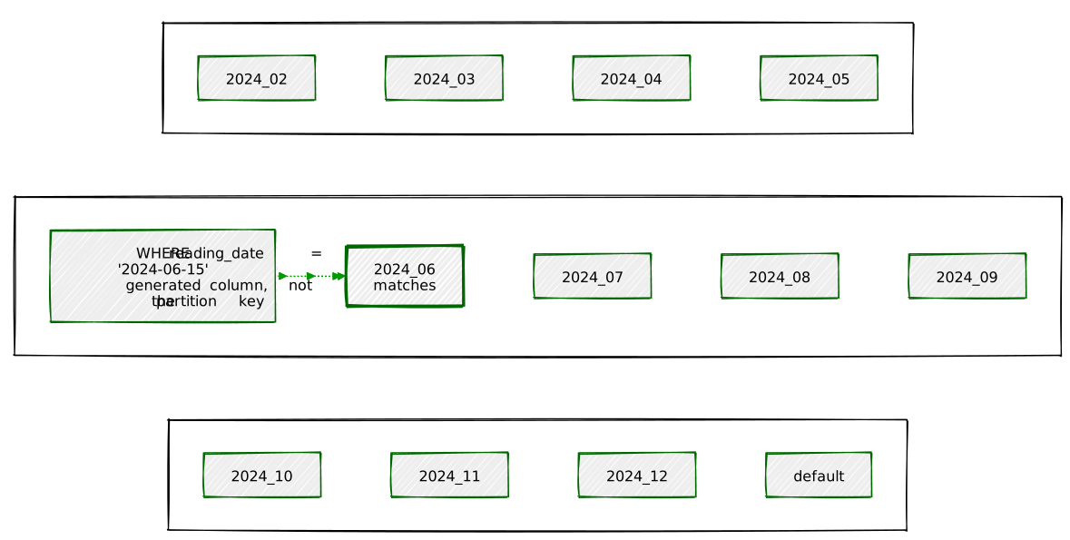
4.1 — Try to UPDATE one
UPDATE sensor_readings SET reading_date = '2020-01-01' WHERE id = 1;ERROR: column "reading_date" can only be updated to DEFAULT
DETAIL: Column "reading_date" is a generated column.4.2 — Try to INSERT one explicitly
INSERT INTO sensor_readings (sensor_id, sensor_type, reading_value, recorded_at, reading_date)
VALUES (1, 'temperature', 50.0, now(), '2020-01-01');ERROR: cannot insert a non-DEFAULT value into column "reading_date"
DETAIL: Column "reading_date" is a generated column.Both rejected, for the same reason: there is no path in PostgreSQL
that lets application code — or a typo, or a well-meaning bulk import
script — set a generated column to anything other than what its
expression computes. This is the guarantee a trigger-maintained column
can never quite make: a trigger stops a normal write path from
getting out of sync, but nothing stops a different write path — a bulk
COPY, a migration script, a DBA fixing something by hand at
2 a.m. — from writing directly to the column and skipping the trigger
entirely. A generated column has no other write path to skip.
5.1 — Real messy data, on purpose
Chapter 15’s contact_info composite type stores
phone as free-form text, and five Portsmith residents now
have it filled in with five different formatting conventions — exactly
the mess a real “phone number” field accumulates over time:
SELECT full_name, (contact).phone FROM residents WHERE id BETWEEN 1 AND 5; full_name | phone
--------------------+------------------
Adrian Foscolo | 023 9281 4477
Marisol Quintero | 023-9281-5522
Bennett Okoye | (023) 9281 6633
Wilhelmina Strand | +44 23 9281 7744
Tobias Renner | 023928188555.2 — Strip everything but the digits
ALTER TABLE residents ADD COLUMN phone_digits TEXT
GENERATED ALWAYS AS (regexp_replace((contact).phone, '[^0-9]', '', 'g')) STORED;SELECT full_name, (contact).phone, phone_digits FROM residents WHERE id BETWEEN 1 AND 5; full_name | phone | phone_digits
--------------------+------------------+---------------
Adrian Foscolo | 023 9281 4477 | 02392814477
Marisol Quintero | 023-9281-5522 | 02392815522
Bennett Okoye | (023) 9281 6633 | 02392816633
Wilhelmina Strand | +44 23 9281 7744 | 442392817744
Tobias Renner | 02392818855 | 02392818855(contact).phone — a field pulled out of Chapter 15’s
composite type — works inside a generated expression exactly like any
other column reference. Four of the five now agree, digit-for-digit,
despite arriving in four visibly different formats.
5.3 — Search with a fifth, still-different format
SELECT full_name FROM residents
WHERE phone_digits = regexp_replace('023.9281.5522', '[^0-9]', '', 'g'); full_name
------------------
Marisol QuinteroA caller can type the number with dots, dashes, spaces, or nothing at all, run it through the identical normalization, and get a match — that’s the entire point of normalizing at write time instead of comparing raw, differently-formatted text.
5.4 — Where this normalization actually stops working
Look at Wilhelmina Strand’s row again: 442392817744, not
02392817744 like everyone else’s. +44 is the
UK’s country code, and 023... is the same number in
domestic format with a leading 0 — the same real phone
number, and this normalization treats them as two different ones,
because stripping non-digit characters has no idea that +44
and a leading 0 mean the same thing. Real phone number
normalization needs an actual phone-numbering-plan library (Python’s
phonenumbers, for instance) that understands country codes,
domestic-format leading digits, and valid-length rules per country —
this exercise’s regexp_replace is the honest, simple
version of the idea, not the production-grade one, the same caution
Chapter 15 gave the email-format domain.
Exercise 2 tore out a trigger and replaced it with a generated column doing the identical job. The comparison worth internalizing, now that you’ve built both:
| Trigger | Generated column | |
|---|---|---|
| Can reference other rows/tables | Yes | No — same row only |
Can have side effects (NOTIFY, logging) |
Yes | No — pure expression only |
| Extra write path can bypass it | Yes — anything that skips the trigger | No — enforced at the column itself |
Shows up in \d as part of the column |
No — hidden in a separate function | Yes — visible in the column definition |
| Recomputed automatically on backfill for existing rows | Only if you remember to run an UPDATE |
Yes — happens as part of ALTER TABLE ADD COLUMN |
A generated column isn’t a strictly better trigger — it’s a
narrower tool that happens to fully cover a specific, common
case: “this column is a pure function of other columns in the same row,
with no side effects.” Chapter 13’s
notify_job_status_change() could never be a generated
column — pg_notify() is a side effect, and the whole point
of that trigger is to reach outside the row it fired on.
search_vector and reading_date never needed to
reach outside their own row at all, which is exactly what made them
convertible. The question worth asking before reaching for either one:
does this derived value ever need to know about anything other than the
row it lives on? If yes, it’s a trigger. If no, it’s a generated column,
and a generated column is simpler in every way that matters once the
answer really is no.
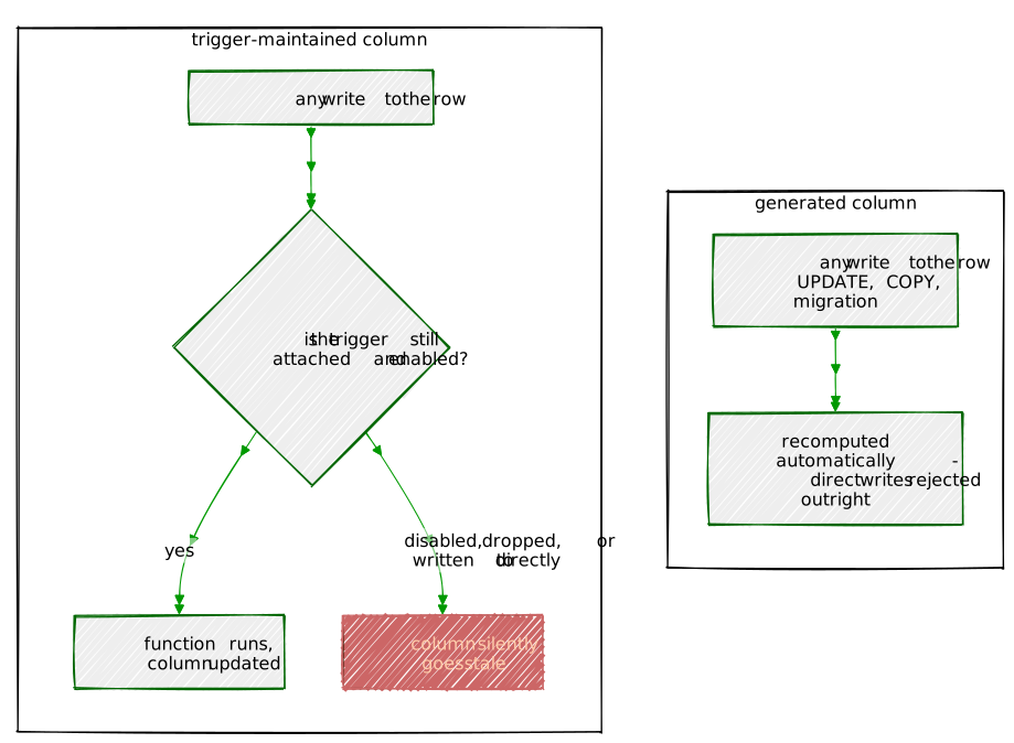
| Tool | What it does |
|---|---|
col type GENERATED ALWAYS AS (expr) STORED |
Computed once at write time, physically stored — the only kind PostgreSQL supports |
| Immutability requirement | The expression can’t depend on session state (timezone, locale) — only on the row’s own columns |
AT TIME ZONE 'UTC' inside the expression |
Fixes the classic ::date immutability failure by
pinning the zone into the expression itself |
| Adding a generated column to an existing table | Backfills every existing row immediately, including every partition of a partitioned table |
DROP COLUMN on a generated column |
Also drops every index that depended on it — rebuild them after |
| Index on a generated column | Used like any other index, subject to the same planner cost decisions (including “seq scan is cheaper on a small table”) |
| Generated column vs. partition key | Indexing a derived column speeds up filtering on it; it does not enable partition pruning, which only ever looks at the actual partition key |
| Writing directly to a generated column | Always rejected — INSERT and UPDATE
both |
| A domain/composite field inside a generated expression | Fully supported — (contact).phone works exactly like
any column reference |
The key design insight from this chapter is the same
one Chapter 15 ended on, aimed at a different part of the schema: a
generated column is a fact about what a value is, not a rule
about what it’s allowed to become after the fact. Chapter 4’s trigger
and this chapter’s search_vector compute the identical
tsvector — but only one of them is structurally incapable
of drifting out of sync, because only one of them removed every write
path except the one that recomputes it correctly. That guarantee has a
real, narrow boundary — no other rows, no side effects, nothing beyond
the current row — and staying inside that boundary is the whole
trade.
Going further: Chapter 17’s foreign data wrappers occasionally
interact with generated columns in an interesting way — a generated
column can’t be added to a foreign table the way it can to a local one,
since PostgreSQL doesn’t control how the remote side actually stores
data. Chapter 20’s pg_stat_statements work is a natural
place to revisit Exercise 3’s planner decision — watching real, measured
query cost is how you’d actually confirm “the planner correctly avoided
the index” rather than taking EXPLAIN’s cost estimate on
faith. And it’s worth remembering Exercise 6’s dividing line the next
time a derived column is on the table at all: reach for a generated
column first, purely for the guarantee it makes, and only fall back to a
trigger once the derivation genuinely needs to see past the row it lives
on.
“A foreign table looks exactly like a table. Everything a DBA would ask before letting you near someone else’s data — do you have the extension, do you have a credential, can you actually reach the file — still has to be answered. It just gets asked in
CREATE SERVERinstead of a ticket queue.”
Every table in this book so far has lived inside
portsmith. A foreign data wrapper (FDW)
lets a table live somewhere else entirely — another PostgreSQL database,
a CSV file on disk, an S3 bucket — while still being queried with
ordinary SELECT, JOIN, and WHERE,
exactly like a local one. No ETL job copies the data in first; the query
reaches out and reads it at query time, through whichever FDW you’ve
told it to use.
The shape is always the same, four pieces:
postgres_fdw,
file_fdw, …) — the driver that knows how to actually talk
to one kind of remote source.portsmith”
says nothing about who you are anywhere else.IMPORT FOREIGN SCHEMA in Exercise 4).
What makes this chapter worth doing hands-on rather than reading
about is that almost none of it works on the first try, and every wall
you hit is a real, deliberate security boundary rather than a bug —
extensions need a privileged role to install, foreign-data wrappers need
explicit USAGE before anyone else can touch them, and a
remote connection needs a real credential even when the same connection
would succeed instantly without one. This chapter hits all three, in
order, exactly where a first-time setup actually hits them.
| Object | Lives in | Purpose |
|---|---|---|
businesses_archive |
portsmith_legacy (a second database) |
Closed Portsmith businesses, pre-migration records |
census_2020.csv |
Server filesystem | 2020 population/household figures, one row per neighbourhood |
legacy_import.businesses_archive |
(built here, via IMPORT FOREIGN SCHEMA) |
The same archive, imported wholesale instead of hand-declared |
sensor_readings/*.parquet |
MinIO bucket portsmith-bucket |
Chapter 8’s full 9.6M-row table, exported one file per month |
portsmith_legacy is a genuinely separate PostgreSQL
database — not a schema inside portsmith — created
specifically to give postgres_fdw something real to reach
across to. Everything in this chapter is a real network round-trip (over
localhost) or a real file read, not a simulation.
By the end of this chapter you will be able to:
postgres_fdw, register a remote PostgreSQL
database as a server, and query one of its tables as if it were local —
and know every privilege that has to be granted along the way, and
why.EXPLAIN, that a WHERE clause
against a foreign table actually executes on the remote server instead
of being pulled over the wire in full.file_fdw, join it
against local data, and know exactly whose filesystem permissions
actually govern whether that works.INSERT, and
verify the row actually landed on the remote server.parquet_s3_fdw
architecture for querying it straight back — what problem it solves, and
what the one genuinely hard-to-install piece still involves.createdb portsmith_legacyIf this fails with permission denied to create database,
your role needs CREATEDB:
-- as postgres
ALTER ROLE your_role CREATEDB;-- as postgres — CREATE EXTENSION requires a privileged role
CREATE EXTENSION postgres_fdw;
CREATE EXTENSION file_fdw;Both ship with core PostgreSQL — no separate package to install, but
creating them requires a role with sufficient privilege, almost always
postgres itself in a development setup like this one.
Only needed if you’re doing the hands-on half of Exercise 6:
source .venv/bin/activate
pip install pyarrow boto3 duckdbIn portsmith_legacy — the “legacy”
archive:
CREATE TABLE businesses_archive (
biz_id INTEGER PRIMARY KEY,
biz_name TEXT NOT NULL,
addr TEXT NOT NULL,
neighbourhood TEXT NOT NULL,
closed_date DATE NOT NULL,
reason TEXT
);
INSERT INTO businesses_archive (biz_id, biz_name, addr, neighbourhood, closed_date, reason) VALUES
(1001, 'Portsmith Cannery Co.', '2 Dock Road', 'Industrial Port', '2011-03-15', 'relocated out of city'),
(1002, 'The Anchor & Rope', '18 Wharf Street', 'Harbour District', '2014-07-01', 'owner retired'),
(1003, 'Old Town Print Shop', '9 Market Street', 'Old Town', '2016-11-30', 'business closed'),
(1004, 'Northgate Ironworks', '44 Bay Street', 'Northgate', '2009-05-20', 'relocated out of city'),
(1005, 'Riverside Boat Repair', '3 Quay Street', 'Riverside', '2018-02-14', 'owner retired'),
(1006, 'University Quarter Bindery', '61 Lighthouse Avenue', 'University Quarter', '2013-09-01', 'business closed'),
(1007, 'Portsmith Rope & Sail', '7 Anchor Lane', 'Harbour District', '2007-01-10', 'merged with another business'),
(1008, 'Dockside Chandlery', '15 Fisherman''s Row', 'Industrial Port', '2019-06-25', 'business closed');On the server filesystem —
data/ch17_census.csv:
neighbourhood,population_2020,households_2020,median_age
Harbour District,8420,3610,41.2
Old Town,6150,2890,44.7
Northgate,11730,4920,36.5
Riverside,9280,3945,39.8
University Quarter,7460,2210,24.3
Industrial Port,5340,2280,45.1-- in portsmith_legacy
SELECT COUNT(*) FROM businesses_archive; count
-------
8postgres_fdw: Server, User Mapping, Foreign Table1.1 — Register the remote server
Back in portsmith:
CREATE SERVER portsmith_legacy_srv
FOREIGN DATA WRAPPER postgres_fdw
OPTIONS (host 'localhost', port '5432', dbname 'portsmith_legacy');If this fails with
permission denied for foreign-data wrapper postgres_fdw,
the role creating the server needs USAGE on the FDW itself
— creating the extension doesn’t automatically hand every other
role the right to use it:
-- as postgres
GRANT USAGE ON FOREIGN DATA WRAPPER postgres_fdw TO your_role;1.2 — Map your local role to a remote identity
CREATE USER MAPPING FOR CURRENT_USER
SERVER portsmith_legacy_srv
OPTIONS (user 'chris');1.3 — Declare the foreign table
CREATE FOREIGN TABLE businesses_archive (
biz_id INTEGER,
biz_name TEXT,
addr TEXT,
neighbourhood TEXT,
closed_date DATE,
reason TEXT
) SERVER portsmith_legacy_srv OPTIONS (schema_name 'public', table_name 'businesses_archive');1.4 — Query it, and hit the gotcha that catches almost everyone
SELECT * FROM businesses_archive ORDER BY biz_id;ERROR: password or GSSAPI delegated credentials required
DETAIL: Non-superusers must delegate GSSAPI credentials or provide a password in the user mapping.This is surprising the first time: the exact same role, over the
exact same localhost connection, can already reach
portsmith_legacy directly with no password prompt at all —
but postgres_fdw refuses to let a non-superuser’s
user mapping ride on that trust. The reasoning is a real security
concern, not bureaucracy: without this check, any role could create a
user mapping claiming to be a powerful remote user and inherit that
user’s privileges on the remote side with nothing to prove it. The fix
is to give the mapping an actual credential:
ALTER ROLE chris PASSWORD 'fdw-demo-password';
ALTER USER MAPPING FOR CURRENT_USER
SERVER portsmith_legacy_srv
OPTIONS (ADD password 'fdw-demo-password');SELECT * FROM businesses_archive ORDER BY biz_id; biz_id | biz_name | addr | neighbourhood | closed_date | reason
--------+-----------------------------+-----------------------+---------------------+-------------+-------------------------------
1001 | Portsmith Cannery Co. | 2 Dock Road | Industrial Port | 2011-03-15 | relocated out of city
1002 | The Anchor & Rope | 18 Wharf Street | Harbour District | 2014-07-01 | owner retired
1003 | Old Town Print Shop | 9 Market Street | Old Town | 2016-11-30 | business closed
1004 | Northgate Ironworks | 44 Bay Street | Northgate | 2009-05-20 | relocated out of city
1005 | Riverside Boat Repair | 3 Quay Street | Riverside | 2018-02-14 | owner retired
1006 | University Quarter Bindery | 61 Lighthouse Avenue | University Quarter | 2013-09-01 | business closed
1007 | Portsmith Rope & Sail | 7 Anchor Lane | Harbour District | 2007-01-10 | merged with another business
1008 | Dockside Chandlery | 15 Fisherman's Row | Industrial Port | 2019-06-25 | business closed
(8 rows)Eight rows, physically stored in a different database, returned by a
plain SELECT with no hint anywhere in the syntax that they
came from anywhere else.
EXPLAIN (VERBOSE)
SELECT biz_name, closed_date FROM businesses_archive WHERE neighbourhood = 'Harbour District'; Foreign Scan on public.businesses_archive (cost=100.00..127.20 rows=7 width=36)
Output: biz_name, closed_date
Remote SQL: SELECT biz_name, closed_date FROM public.businesses_archive WHERE ((neighbourhood = 'Harbour District'))Remote SQL is the whole point: postgres_fdw
didn’t pull all eight rows to portsmith and filter them
here. It translated the query — WHERE, and only the two
selected columns — into real SQL, sent it to
portsmith_legacy, and let that server do the filtering with
its own planner and its own (in a real deployment) indexes. Every row
that doesn’t match Harbour District never crosses the network at
all.
file_fdw: a CSV as a Table3.1 — Server and foreign table
CREATE SERVER census_files FOREIGN DATA WRAPPER file_fdw;
CREATE FOREIGN TABLE census_2020 (
neighbourhood TEXT,
population_2020 INTEGER,
households_2020 INTEGER,
median_age NUMERIC
) SERVER census_files OPTIONS (
filename '/home/you/book/data/ch17_census.csv', -- your actual checkout path
format 'csv',
header 'true'
);If this fails with
permission denied to set the "filename" option,
file_fdw restricts which roles can point a foreign table at
an arbitrary local file — for good reason, since it would otherwise let
any role read anything the PostgreSQL server process itself can
read:
-- as postgres
GRANT pg_read_server_files TO your_role;3.2 — The gotcha that actually matters: whose filesystem is this?
SELECT * FROM census_2020;ERROR: could not open file "/home/you/book/data/ch17_census.csv" for reading: Permission deniedThe client running psql can read this file fine — but
file_fdw doesn’t read the file from the client. It reads it
from the server process, running as its own OS user
(postgres, typically), and that user has to have its own
filesystem path to the file, readable by it, independent of
who’s connected. A file sitting inside a user’s home directory — mode
700 by default on most systems — is invisible to every
other OS user no matter what the file’s own permissions say, because the
directory blocks entry before the file’s permissions ever get
checked. The fix isn’t to loosen a home directory’s permissions; it’s to
put the file somewhere server-readable in the first place —
/tmp for a throwaway demo like this one, a dedicated data
directory with the right ownership for anything real:
cp data/ch17_census.csv /tmp/ch17_census.csv
chmod 644 /tmp/ch17_census.csvALTER FOREIGN TABLE census_2020 OPTIONS (SET filename '/tmp/ch17_census.csv');
SELECT * FROM census_2020; neighbourhood | population_2020 | households_2020 | median_age
----------------------+------------------+------------------+------------
Harbour District | 8420 | 3610 | 41.2
Old Town | 6150 | 2890 | 44.7
Northgate | 11730 | 4920 | 36.5
Riverside | 9280 | 3945 | 39.8
University Quarter | 7460 | 2210 | 24.3
Industrial Port | 5340 | 2280 | 45.1
(6 rows)3.3 — Join it against local data
SELECT c.neighbourhood, c.population_2020, COUNT(b.id) AS business_count
FROM census_2020 c
JOIN businesses b ON b.neighbourhood = c.neighbourhood
GROUP BY c.neighbourhood, c.population_2020
ORDER BY c.population_2020 DESC; neighbourhood | population_2020 | business_count
----------------------+------------------+-----------------
Northgate | 11730 | 9
Riverside | 9280 | 9
Harbour District | 8420 | 9
University Quarter | 7460 | 5
Old Town | 6150 | 9
Industrial Port | 5340 | 7
(6 rows)A flat file and a real table, joined with ordinary SQL — nothing
about the query syntax distinguishes census_2020 (a CSV)
from businesses (an actual table).
3.4 — The contrast with Exercise 2: no pushdown here
EXPLAIN SELECT * FROM census_2020 WHERE neighbourhood = 'Northgate'; Foreign Scan on census_2020 (cost=0.00..1.21 rows=1 width=72)
Filter: (neighbourhood = 'Northgate'::text)
Foreign File: /tmp/ch17_census.csvFilter:, not Remote SQL:. A flat file has
no query engine of its own to push anything down to —
file_fdw has no choice but to read every row of the file
into PostgreSQL and filter locally, every time. For a six-row census
file that’s irrelevant; for a multi-gigabyte CSV it’s the entire
performance story, and it’s the exact gap Exercise 6’s
parquet_s3_fdw pattern exists to close.
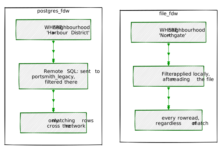
Exercise 1 declared businesses_archive by hand, column
by column — fine for one table, tedious for a real legacy database with
dozens. IMPORT FOREIGN SCHEMA asks the remote server for
its own schema and generates matching foreign tables automatically:
CREATE SCHEMA legacy_import;
IMPORT FOREIGN SCHEMA public
FROM SERVER portsmith_legacy_srv
INTO legacy_import;\d legacy_import.businesses_archive Foreign table "legacy_import.businesses_archive"
Column | Type | Collation | Nullable | Default | FDW options
----------------+---------+-----------+----------+---------+--------------------------------
biz_id | integer | | not null | | (column_name 'biz_id')
biz_name | text | | not null | | (column_name 'biz_name')
addr | text | | not null | | (column_name 'addr')
neighbourhood | text | | not null | | (column_name 'neighbourhood')
closed_date | date | | not null | | (column_name 'closed_date')
reason | text | | | | (column_name 'reason')
Server: portsmith_legacy_srvEvery column, every type, matched exactly — not retyped by hand, read
directly off the remote catalog. IMPORT FOREIGN SCHEMA also
accepts LIMIT TO (...) or EXCEPT (...) clauses
to import only part of a schema, worth knowing the moment a real legacy
database has hundreds of tables and you need eight of them.
INSERT INTO businesses_archive (biz_id, biz_name, addr, neighbourhood, closed_date, reason)
VALUES (1009, 'Old Brewery Annex', '12 Ring Road', 'Industrial Port', '2021-08-30', 'demolished for redevelopment');INSERT 0 1Verify it landed on the actual remote database, not just in a local cache:
-- connect directly to portsmith_legacy
SELECT biz_id, biz_name FROM businesses_archive WHERE biz_id = 1009; biz_id | biz_name
--------+--------------------
1009 | Old Brewery AnnexA plain INSERT against portsmith, and the
row is sitting in portsmith_legacy —
postgres_fdw supports writes as well as reads, translated
into a real INSERT on the remote side, subject to every
constraint that database enforces on its own table (a duplicate
biz_id would fail here exactly as it would connecting
directly). file_fdw cannot do this — a CSV file has no
transactional write protocol to translate an INSERT into,
and Chapter 17’s file-based foreign tables are read-only for exactly
that reason.
parquet_s3_fdw Pattern6.1 — The problem this solves
sensor_readings (Chapter 8) is 9.6 million rows and only
grows. Most of it, most of the time, is cold — nobody’s actively
querying January’s readings in November. Keeping years of it in
PostgreSQL forever is possible but not free: it’s backed up on every
backup, it’s vacuumed on every autovacuum pass, it occupies disk that
costs money whether or not anyone reads it. A common real-world answer
is to export aging partitions out of PostgreSQL entirely into
Parquet — a columnar file format built for exactly
this: cheap object storage (S3 or, for local development, an
S3-compatible server like MinIO), with per-column
compression and the ability to skip whole chunks of a file that can’t
possibly match a filter, without reading them.
The catch that would normally follow: exporting the data means it’s
no longer queryable with plain SQL, from the same connection, joined
against whatever’s still live in PostgreSQL. parquet_s3_fdw
closes that gap — a foreign data wrapper that reads Parquet files
sitting in S3-compatible storage as ordinary foreign tables, pushing
down both column selection and predicate filtering into the Parquet
reader itself (Parquet’s own format stores per-column statistics,
min/max values per row group, that let a reader skip entire chunks
without decompressing them — a real analog to
postgres_fdw’s Remote SQL pushdown from
Exercise 2, just implemented against a file format instead of a second
database).
6.2 — The half of this that’s completely real: export and upload
Getting data into Parquet, in S3-compatible storage, needs
nothing exotic — pyarrow to write the files,
boto3 (or any S3-compatible client) to upload them, and
MinIO running locally in Docker to receive them:
docker run -p 9000:9000 -p 9001:9001 minio/minio server /data --console-address ":9001"#!/usr/bin/env python3.12
# ch17_export_to_parquet.py — one Parquet file per monthly partition
import io
from datetime import date, timedelta
import boto3
import psycopg
import pyarrow as pa
import pyarrow.parquet as pq
MINIO_ENDPOINT, MINIO_ACCESS_KEY, MINIO_SECRET_KEY = "http://localhost:9000", "minioadmin", "minioadmin"
BUCKET = "portsmith-bucket"
QUERY = """
SELECT sensor_id, sensor_type, reading_value, recorded_at, reading_date
FROM sensor_readings
WHERE reading_date >= %(start)s AND reading_date < %(end)s
ORDER BY recorded_at
"""
def export_month(conn, year_month: str) -> pa.Table:
year, month = (int(p) for p in year_month.split("-"))
start = date(year, month, 1)
end = (date(year, month + 1, 1) if month < 12 else date(year + 1, 1, 1))
with conn.cursor() as cur:
cur.execute(QUERY, {"start": start, "end": end})
rows = cur.fetchall()
cols = ["sensor_id", "sensor_type", "reading_value", "recorded_at", "reading_date"]
return pa.table({c: [r[i] for r in rows] for i, c in enumerate(cols)})
# ... build an S3 client pointed at MINIO_ENDPOINT, create the bucket if
# needed, then for each month: export_month(), pq.write_table() into an
# in-memory buffer, s3.upload_fileobj() to sensor_readings/{month}.parquetRun against all of sensor_readings’ eleven populated
months:
2024-02: 835,200 rows -> s3://portsmith-bucket/sensor_readings/2024-02.parquet (1,420,131 bytes)
2024-03: 892,800 rows -> s3://portsmith-bucket/sensor_readings/2024-03.parquet (1,540,196 bytes)
...
2024-12: 891,648 rows -> s3://portsmith-bucket/sensor_readings/2024-12.parquet (1,527,345 bytes)
done — 9,646,849 rows, 16,673,067 bytes across 11 files9.6 million real rows, genuinely uploaded to genuinely running
S3-compatible storage, in under three minutes. And the number worth
sitting with: sensor_readings occupies 772
MB in PostgreSQL (table plus every index, summed across all its
partitions); the same data, as Parquet with Snappy compression, is
16.7 MB — about 46 times smaller. That
gap is column-oriented storage and per-column compression doing exactly
what they’re for: sensor_readings has five columns, several
of them low-cardinality (sensor_type is one of three
values, repeated 9.6 million times) or smoothly-changing
(recorded_at, reading_date), and a columnar
format compresses runs of similar values far more efficiently than a
row-oriented table ever will.
6.3 — The half of this chapter that stays a sketch: the FDW itself
Querying these files back from PostgreSQL — the actual
parquet_s3_fdw part — is where this exercise stops being
fully hands-on. It isn’t a core PostgreSQL extension the way
postgres_fdw and file_fdw are; it’s a
third-party project built against Apache Arrow’s C++ libraries, compiled
from source in most environments rather than installed with
apt. Getting a working build means matching Arrow/Parquet
library versions to your exact PostgreSQL version, a real, multi-step
undertaking well outside what a single exercise can responsibly walk
through. What follows is the setup this chapter would ask you to do if
it did — worth understanding piece by piece, and worth treating as a
genuine follow-on project now that the data is actually sitting in MinIO
waiting for it:
parquet_s3_fdw
against your PostgreSQL version’s server headers.CREATE SERVER, pointing at the MinIO
endpoint instead of a PostgreSQL host — an access key and secret in
place of a username and password, the S3 analog of Exercise 1’s user
mapping.CREATE FOREIGN TABLE (or
IMPORT FOREIGN SCHEMA, if the extension supports inferring
the Parquet schema — implementations vary), mapping Parquet columns the
same way Exercise 4 mapped a remote PostgreSQL table’s columns.WHERE reading_date = '2024-06-15' against all eleven
exported files should skip most of their row groups entirely, the same
shape of win Exercise 2’s Remote SQL pushdown demonstrated,
just decided by Parquet’s own per-column statistics instead of a remote
query planner.The architecture, end to end: PostgreSQL stays the single query
interface for both hot data (still in sensor_readings) and
cold data (exported to Parquet in MinIO/S3, exactly as Exercise 6.2 just
did for real), joinable in the same query, without standing up a
separate query engine like Trino or Presto just to read files a data
lake already has sitting in object storage.
6.4 — Verifying the pruning story independently, with DuckDB
parquet_s3_fdw isn’t the only thing that can read
Parquet off S3-compatible storage — DuckDB can too,
natively, and installing it is one pip install duckdb
rather than a source build. It’s a useful second opinion here: query the
exported files directly, with no PostgreSQL involved at all, and confirm
the row-group pruning story Exercise 6.1 promised is actually true.
#!/usr/bin/env python3.12
# ch17_query_parquet.py
import duckdb
con = duckdb.connect()
con.execute("INSTALL httpfs; LOAD httpfs;")
con.execute("""
SET s3_endpoint = 'localhost:9000';
SET s3_access_key_id = 'minioadmin';
SET s3_secret_access_key = 'minioadmin';
SET s3_use_ssl = false;
SET s3_url_style = 'path';
""")
GLOB = "s3://portsmith-bucket/sensor_readings/*.parquet"
print(con.execute(f"SELECT COUNT(*) FROM read_parquet('{GLOB}')").fetchone())
con.execute(f"""
EXPLAIN ANALYZE SELECT COUNT(*) FROM read_parquet('{GLOB}')
WHERE reading_date = DATE '2024-06-15'
""")
for row in con.fetchall():
print(row[1])(9646849,)Nine million, six hundred forty-six thousand, eight hundred forty-nine — matching Exercise 6.2’s own upload total exactly, confirming nothing was lost or duplicated across eleven separate uploads. Then the pruning check:
HTTPFS HTTP Stats
in: 2.7 KiB
out: 0 bytes
#GET: 1
Total Time: 0.0048s
TABLE_SCAN (READ_PARQUET)
Filters: reading_date='2024-06-15':DATE
Total Files Read: 11
28,801 rows2.7 KiB of actual data transferred, one HTTP
GET, to answer a query that matched 28,801 rows — out of
16.7 MB and 9.6 million rows total. Total Files Read: 11
looks like it contradicts that at first — DuckDB did open every
file — but opening a Parquet file only costs reading its footer, a small
block of per-row-group statistics; the actual column data for row groups
that can’t contain 2024-06-15 never gets requested at all.
(This number reflects the two queries that ran before it in the same
session already having warmed DuckDB’s metadata cache for these files —
a cold connection running only the EXPLAIN ANALYZE query
would transfer somewhat more, closer to 180 KiB, still a small fraction
of the total.) Either way, this is Exercise 2’s Remote SQL
pushdown story again, a third time in one chapter: a system that
understands the shape of its own storage well enough to answer “which
parts of this can I skip” before reading them.
Every wall this chapter actually hit, in the order it hit them:
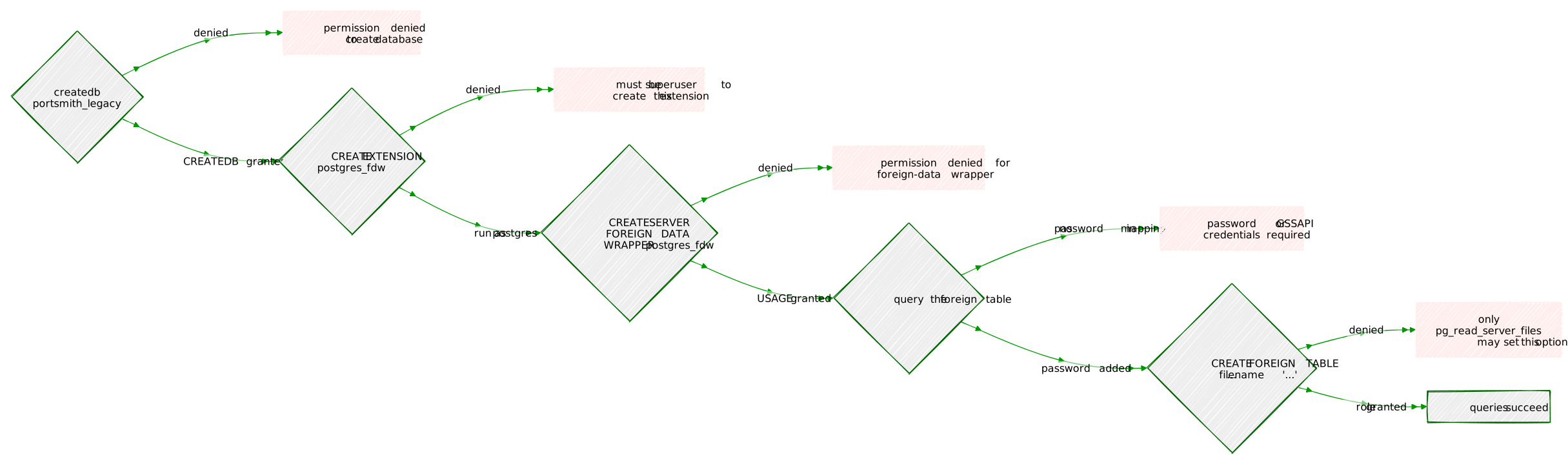
| Tool | What it does |
|---|---|
CREATE EXTENSION postgres_fdw /
file_fdw |
Installs the driver — requires a privileged role |
GRANT USAGE ON FOREIGN DATA WRAPPER ... TO role |
Required before a non-privileged role can create a server with that FDW |
CREATE SERVER |
Registers one remote endpoint under a name |
CREATE USER MAPPING |
Maps a local role to a remote identity — non-superusers must supply a real password |
CREATE FOREIGN TABLE |
Declares a local name for a remote shape of data, column by column |
IMPORT FOREIGN SCHEMA ... INTO schema |
Generates foreign tables for an entire remote schema automatically |
EXPLAIN on a foreign table
(postgres_fdw) |
Remote SQL: — confirms filtering happened on the remote
server, not locally |
EXPLAIN on a foreign table (file_fdw) |
Filter: — confirms the whole file was read and filtered
locally instead |
pg_read_server_files |
The role membership file_fdw requires before pointing
at an arbitrary local file |
File permissions for file_fdw |
Governed by the PostgreSQL server process’s OS user, not the connecting client |
INSERT through a postgres_fdw foreign
table |
A real write, translated and executed on the remote server |
parquet_s3_fdw |
Same pattern as postgres_fdw, aimed at columnar files
in S3-compatible storage instead of another database |
The key design insight from this chapter is that a
foreign data wrapper’s job is to make remote data look exactly
like local data — and it succeeds completely at that, right up until you
touch something that was never really local to begin with: a credential,
a filesystem permission, a network round-trip. Every gotcha this chapter
walked through was one of those seams showing through the illusion on
purpose, not by accident — PostgreSQL enforcing, at each layer, that
querying someone else’s data still has to answer the same questions it
always would have, just inside CREATE SERVER and
CREATE USER MAPPING instead of a separate integration layer
you’d otherwise have to build and maintain by hand.
Going further: Chapter 18’s logical replication solves a related
but genuinely different problem — where this chapter queries remote data
live, at read time, replication copies* it, continuously, so a
second database has its own independent, current copy to query locally.
Reach for an FDW when the data should stay in one place and be reached
across; reach for replication when a second copy, kept in sync, is what
you actually need. And Exercise 6’s parquet_s3_fdw sketch
is worth revisiting once Chapter 19’s pg_cron is in hand —
a scheduled job that exports aging sensor_readings
partitions to Parquet and drops them locally, the same way Chapter 8’s
own “going further” note imagined pg_partman automating
partition lifecycle management, is exactly the kind of recurring
maintenance pg_cron is suited to run unattended.*
A foreign data wrapper asks a question and waits for an answer, every time. A subscription asks once, then never stops listening.
Every business and permit in Portsmith lives in one place:
portsmith, the operational database every clerk’s terminal
and every intake job reads and writes directly. That’s exactly where it
should live — until the city decides it also wants a public-facing
Business Finder portal, so a resident can search
“what’s open in Old Town” or check whether their neighbor’s demolition
permit has cleared, without calling City Hall.
Pointing the portal straight at portsmith — a live
connection, or Chapter 17’s postgres_fdw reaching across at
query time — is the obvious first idea, and IT rejects it fast. A
Saturday-morning traffic spike on the public site has no business
competing for locks and connections with a clerk mid-edit on a permit.
The portal also has no business seeing everything portsmith
has: no PostGIS geometry, no internal search-ranking internals, and
definitely nothing from businesses that have since closed. And a nightly
export job — the other obvious idea — means a business that reopens
Tuesday morning doesn’t show as open on the portal until Wednesday’s
batch run, which isn’t good enough for something citizens are expected
to trust.
What the city actually wants is a second, independent copy of just
the public-facing slice of businesses and jobs
— one the portal can hit as hard as it likes without touching the real
system, that only ever shows currently-active businesses, and that
updates itself the moment something changes upstream, with nobody
babysitting a cron job. Logical replication is exactly
that: it streams every row-level change out of PostgreSQL, continuously,
so a second database ends up with its own current copy — queryable
locally, with its own indexes, filtered down to only the columns and
rows that copy is allowed to see. Experientially, once it’s running, it
disappears: a clerk approves a new registration in
portsmith, and a moment later — no refresh button, no
scheduled job, nobody polling anything — that business is searchable on
the portal. This chapter builds the portal’s copy as
portsmith_legacy, the same second database Chapter 17
introduced, now playing a different role: instead of something
portsmith reaches into, it’s something
portsmith continuously pushes into.
The mechanism underneath is the same write-ahead log
(WAL) every PostgreSQL install already produces for crash
recovery, decoded into a stream of logical changes (INSERT,
UPDATE, DELETE) instead of the physical
byte-level records physical replication (streaming
standbys) sends. Two pieces make it work:
Underneath every subscription is a replication slot — a durable bookmark on the publisher that says “don’t let WAL older than this be recycled, a consumer still needs it.” That’s the whole safety contract: as long as the slot exists, the publisher retains whatever WAL the subscriber hasn’t confirmed yet, even across a subscriber outage. It’s also the whole risk: a slot nobody’s draining anymore retains WAL forever, silently filling disk.
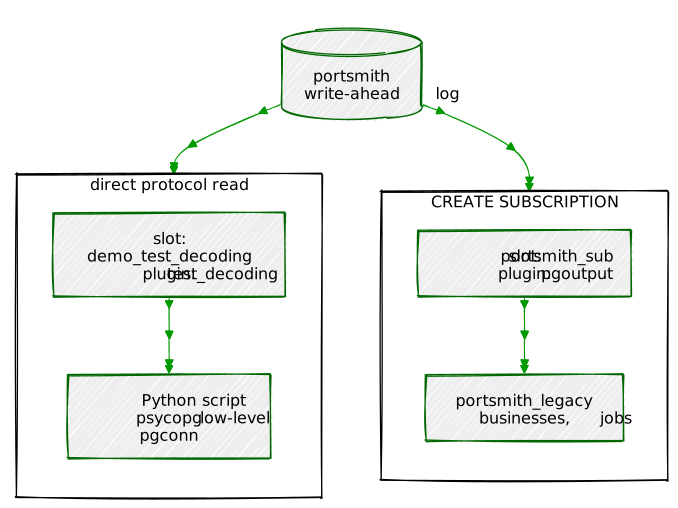
This chapter builds both paths off the same publisher: the standard
CREATE SUBSCRIPTION route or the second row shows the raw
protocol, read directly from Python.
| Object | Lives in | Purpose |
|---|---|---|
portsmith_pub |
portsmith (publisher) |
Publication covering businesses (partial columns,
row-filtered) and jobs (all columns) |
portsmith_sub |
portsmith_legacy (subscriber) |
Subscription consuming portsmith_pub, backed by a slot
of the same name on the publisher |
businesses / jobs |
Both databases | Chapter 1 / Chapter 3’s tables — subscriber’s copies are narrower, no PostGIS geometry, no generated columns |
demo_test_decoding |
portsmith (publisher) |
A second, independent slot, read directly by Python instead of by a subscription |
data/ch18_replication_stream.py |
(new) | Consumes demo_test_decoding at the wire protocol
level |
portsmith_legacy is the same second database Chapter 17
created — now standing in for the Business Finder portal’s own database,
on the same PostgreSQL instance as the publisher. That’s convenient for
a lab environment and, as Exercise 2 shows, not free: it creates a real
deadlock a genuinely separate instance (which is what a real portal
database would be) wouldn’t.
By the end of this chapter you will be able to:
pg_replication_slots and
pg_stat_replication to check lag and confirm a subscriber
is actually keeping up.CREATE SUBSCRIPTION at all.wal_level = logicalLogical decoding needs more information in the WAL than PostgreSQL writes by default:
-- as postgres, in postgresql.conf, or:
ALTER SYSTEM SET wal_level = 'logical';# postgresql.conf
wal_level = logical # (change requires restart)Like shared_preload_libraries in the previous two
chapters’ setup, this needs a full restart, not just a config
reload:
sudo systemctl restart postgresqlSHOW wal_level; wal_level
-----------
logicalNo other extension is needed — logical replication is built into core PostgreSQL.
portsmith_legacy needs matching structure for whatever
gets published, but matching doesn’t mean identical.
businesses in portsmith carries a PostGIS
geometry column and a generated tsvector —
neither makes sense to replicate here: portsmith_legacy has
no PostGIS extension installed, and generated columns aren’t sent over
logical replication anyway (PostgreSQL 16 excludes them from the wire
format by default; a subscriber with the same generated column would
just compute its own value locally, and one without it simply doesn’t
have it). So the subscriber’s businesses is deliberately
narrower — the domain and enum types still have to match, since those
govern the columns that are published:
-- in portsmith_legacy
CREATE DOMAIN positive_integer AS integer CHECK (VALUE > 0);
CREATE TYPE job_status AS ENUM ('queued','on_hold','in_progress','completed','failed','cancelled');
CREATE TABLE businesses (
id integer PRIMARY KEY,
name text NOT NULL,
address text NOT NULL,
neighbourhood text NOT NULL,
details jsonb NOT NULL,
employee_count positive_integer
);
CREATE TABLE jobs (
id bigint PRIMARY KEY,
job_type text NOT NULL,
payload jsonb NOT NULL,
status job_status NOT NULL DEFAULT 'queued',
priority smallint NOT NULL DEFAULT 5,
attempts integer NOT NULL DEFAULT 0,
max_attempts integer NOT NULL DEFAULT 3,
created_at timestamptz NOT NULL DEFAULT clock_timestamp(),
claimed_at timestamptz,
claimed_by text,
heartbeat_at timestamptz,
completed_at timestamptz,
last_error text
);jobs is published in full — no PostGIS-shaped
complications there, so its subscriber copy is a plain structural
match.
wal_level and a PublicationWith wal_level already set to logical,
creating a publication is the easy part:
-- in portsmith
CREATE PUBLICATION portsmith_pub
FOR TABLE businesses (id, name, address, neighbourhood, details, employee_count), jobs;CREATE PUBLICATIONbusinesses uses a column list —
PostgreSQL 15+ lets a publication name a subset of a table’s columns,
not just a subset of its rows. Here that’s what makes the narrower
subscriber schema above valid at all: geom and
search_vector are simply never offered, so
portsmith_legacy never needs to know they exist.
Practically, this is the city deciding what the portal is
allowed to see: internal geometry and search-ranking internals
stay behind in portsmith, never even leaving the
publisher’s WAL decode step for this publication.
SELECT pubname, puballtables FROM pg_publication;
SELECT schemaname, tablename, attnames FROM pg_publication_tables WHERE pubname = 'portsmith_pub'; pubname | puballtables
----------------------+---------------
portsmith_pub | f
schemaname | tablename | attnames
------------+------------+--------------------------------------------------------------
public | businesses | {id,name,address,neighbourhood,details,employee_count}
public | jobs | {id,job_type,payload,status,priority,attempts,max_attempts,created_at,claimed_at,claimed_by,heartbeat_at,completed_at,last_error}2.1 — Two permission gates, back to back
-- in portsmith_legacy
CREATE SUBSCRIPTION portsmith_sub
CONNECTION 'host=localhost dbname=portsmith user=chris password=fdw-demo-password'
PUBLICATION portsmith_pub;ERROR: permission denied to create subscription
DETAIL: Only roles with privileges of the "pg_create_subscription" role may create subscriptions.A PostgreSQL 16 hardening measure — creating a subscription can execute arbitrary code on the publisher’s behalf (via the connection string), so it’s gated behind its own predefined role, separate from ordinary table privileges:
-- as postgres
GRANT pg_create_subscription TO chris;Retrying reaches a second, unrelated gate:
ERROR: could not connect to the publisher: connection to server at "localhost" (127.0.0.1), port 5432 failed: FATAL: permission denied to start WAL sender
DETAIL: Only roles with the REPLICATION attribute may start a WAL sender process.pg_create_subscription governs creating the
local subscription object; actually connecting to the publisher
and opening a replication connection is gated separately, by a role
attribute (like LOGIN or CREATEDB),
not a grantable role membership:
-- as postgres
ALTER ROLE chris REPLICATION;2.2 — The deadlock
Retrying again:
CREATE SUBSCRIPTION portsmith_sub
CONNECTION 'host=localhost dbname=portsmith user=chris password=fdw-demo-password'
PUBLICATION portsmith_pub;…hangs. No error, no completion — indefinitely. From another session:
SELECT l.pid, l.mode, l.granted, a.query
FROM pg_locks l JOIN pg_stat_activity a ON a.pid = l.pid
WHERE l.locktype = 'transactionid'; pid | mode | granted | query
--------+---------------+---------+------------------------------------------------------------
322315 | ExclusiveLock | t | CREATE SUBSCRIPTION portsmith_sub CONNECTION ... ;
322316 | ShareLock | f | CREATE_REPLICATION_SLOT "portsmith_sub" LOGICAL pgoutput (SNAPSHOT 'nothing')CREATE SUBSCRIPTION (pid 322315), by default, tries to
create its replication slot as part of its own work — and creating a
logical slot needs a consistent snapshot, which means waiting
for every other currently-running transaction in the cluster to finish.
Because the publisher and subscriber are the same PostgreSQL
instance here, the walsender process it spawns to build that
snapshot (pid 322316) ends up waiting on
CREATE SUBSCRIPTION’s own, still-open transaction
— which can’t finish until the slot creation it’s waiting on returns. A
true self-deadlock, specific to same-instance publisher/subscriber
setups; a genuinely separate PostgreSQL server wouldn’t have this
problem, since its walsender would never need to wait on a transaction
ID that belongs to a different cluster entirely.
Cancel it and clean up:
SELECT pg_cancel_backend(322315);2.3 — The real fix: create the slot first, separately
-- in portsmith (the publisher)
SELECT pg_create_logical_replication_slot('portsmith_sub', 'pgoutput'); pg_create_logical_replication_slot
-------------------------------------
(portsmith_sub,0/C697AEB8)-- in portsmith_legacy
CREATE SUBSCRIPTION portsmith_sub
CONNECTION 'host=localhost dbname=portsmith user=chris password=fdw-demo-password'
PUBLICATION portsmith_pub
WITH (create_slot = false, slot_name = 'portsmith_sub');CREATE SUBSCRIPTIONWith the slot already sitting there, CREATE SUBSCRIPTION
has nothing left to wait on — it just starts the initial data copy
immediately:
SELECT count(*) FROM businesses; -- in portsmith_legacy
SELECT count(*) FROM jobs; count count
------- -------
48 482.4 — Real-time replication
-- in portsmith
INSERT INTO businesses (name, address, neighbourhood, details, employee_count)
VALUES ('Harbor Light Cafe', '12 Quay Street', 'Old Town', '{"category":"restaurant"}', 6)
RETURNING id;-- moments later, in portsmith_legacy
SELECT id, name, employee_count FROM businesses WHERE name = 'Harbor Light Cafe'; id | name | employee_count
----+--------------------+-----------------
49 | Harbor Light Cafe | 6No polling, no manual refresh — the row is there because a walsender
process pushed it the moment the INSERT committed on the
publisher. This is the payoff the whole chapter is built around: a clerk
enters Harbor Light Cafe’s registration in portsmith, and —
with nobody running a sync script, no nightly job, nothing on a timer —
it’s already sitting in the portal’s own database, ready for the next
citizen search.
This is the question an operator actually asks about the Business Finder portal: is it still current, or has it quietly fallen behind without anyone noticing? These two views are how you’d answer that — in a monitoring dashboard, not just by hand.
-- in portsmith
SELECT slot_name, plugin, slot_type, database, active, restart_lsn, confirmed_flush_lsn
FROM pg_replication_slots; slot_name | plugin | slot_type | database | active | restart_lsn | confirmed_flush_lsn
---------------+----------+-----------+-----------+--------+-------------+----------------------
portsmith_sub | pgoutput | logical | portsmith | t | 0/C698E388 | 0/C698E3C0pg_stat_replication is the live, moment-to-moment view —
but querying it as chris at first shows an odd,
mostly-empty row:
SELECT application_name, state, sent_lsn, replay_lsn, replay_lag FROM pg_stat_replication; application_name | state | sent_lsn | replay_lsn | replay_lag
------------------+-------+----------+------------+------------
portsmith_sub | | | |The row exists — chris can see that a
replication connection is active — but the detail columns
(state, every LSN, lag) are hidden unless the querying role
is a superuser or holds pg_monitor:
-- as postgres
GRANT pg_monitor TO chris;SELECT application_name, state, sent_lsn, write_lsn, flush_lsn, replay_lsn, replay_lag
FROM pg_stat_replication; application_name | state | sent_lsn | write_lsn | flush_lsn | replay_lsn | replay_lag
------------------+-----------+------------+------------+------------+------------+------------------
portsmith_sub | streaming | 0/C698EFC8 | 0/C698EFC8 | 0/C698EFC8 | 0/C698EFC8 | 00:00:00.00025state: streaming and a quarter-millisecond
replay_lag — on localhost, replication lag is
essentially the cost of a context switch. The same query against a
subscriber across a real network would show it rising under load, which
is exactly what an operator watches this view for.
A citizen searching the Business Finder portal for a seafood
restaurant in Old Town doesn’t want three shuttered storefronts in the
results. The column list in Exercise 1 controlled what the
portal sees about each business; this exercise controls which
businesses it sees at all — closed ones simply shouldn’t exist as
far as portsmith_legacy is concerned.
4.1 — Give businesses something to filter
on
-- in portsmith
ALTER TABLE businesses ADD COLUMN active boolean NOT NULL DEFAULT true;
UPDATE businesses SET active = false WHERE id IN (6, 8, 14); -- closed since the seed data was written-- in portsmith_legacy, so the published column list still has somewhere to land
ALTER TABLE businesses ADD COLUMN active boolean NOT NULL DEFAULT true;4.2 — Add the filter
-- in portsmith
ALTER PUBLICATION portsmith_pub
SET TABLE businesses (id, name, address, neighbourhood, details, employee_count, active) WHERE (active = true),
jobs;ALTER PUBLICATION4.3 — A refresh alone doesn’t retroactively resync
-- in portsmith_legacy
ALTER SUBSCRIPTION portsmith_sub REFRESH PUBLICATION WITH (copy_data = true);
SELECT count(*) FROM businesses; count
-------
49Still 49 — the three closed businesses are still sitting there, and
still show active = true locally.
REFRESH PUBLICATION only reconciles which tables a
subscription tracks (picking up newly added or removed ones); it does
nothing for a column list or row filter that changed on a table the
subscription is already happily synchronized with. Nothing is wrong —
this is documented behavior, just an easy assumption to get wrong the
first time.
4.4 — Forcing a real resync
ALTER SUBSCRIPTION portsmith_sub DISABLE;
TRUNCATE businesses;
TRUNCATE jobs; -- every table touched by the resync, not just the one you changed
ALTER SUBSCRIPTION portsmith_sub ENABLE;
ALTER SUBSCRIPTION portsmith_sub REFRESH PUBLICATION WITH (copy_data = true);SELECT count(*) FROM businesses;
SELECT id, name FROM businesses WHERE id IN (6, 8, 14); count
-------
46
id | name
----+------
(0 rows)Forty-six — 49 minus the three now-active = false rows —
and none of the closed businesses present at all. Truncate every
table the resync touches, not just the one whose filter
changed. Forgetting one leaves its tablesync worker retrying a
COPY into a table that already has the same primary keys,
forever:
ERROR: duplicate key value violates unique constraint "jobs_pkey"
CONTEXT: COPY jobs, line 1
LOG: logical replication table synchronization worker for subscription "portsmith_sub", table "jobs" has started
... (repeats every ~5 seconds)— a real failure mode, not a hypothetical: exactly this happened while preparing this chapter, from truncating one table in a multi-table resync and not the other.
4.5 — Filtering on a non-key column has its own wall
With the resync clean, flip a business’s active flag
live:
UPDATE businesses SET active = false WHERE id = 49;ERROR: cannot update table "businesses"
DETAIL: Column used in the publication WHERE expression is not part of the replica identity.For an UPDATE, PostgreSQL has to know whether the
old row matched the filter (to decide whether the subscriber
needs a delete-equivalent) — and by default, only the primary key
travels in the WAL as the “old” row image. active isn’t
part of that. The obvious-looking fix:
ALTER TABLE businesses REPLICA IDENTITY FULL;
UPDATE businesses SET active = false WHERE id = 49;ERROR: cannot update table "businesses"
DETAIL: Column list used by the publication does not cover the replica identity.REPLICA IDENTITY FULL swings too far the other way: now
the replica identity is every column, including
geom and search_vector — neither of which the
publication’s column list includes. The real fix is a replica identity
that’s exactly as wide as it needs to be:
CREATE UNIQUE INDEX idx_businesses_replident ON businesses (id, active);
ALTER TABLE businesses REPLICA IDENTITY USING INDEX idx_businesses_replident;UPDATE businesses SET active = false WHERE id = 49;UPDATE 1-- moments later, in portsmith_legacy
SELECT id FROM businesses WHERE id = 49; id
----
(0 rows)Gone — correctly filtered out the moment active flipped,
effectively replicated as a delete. That’s the portal experience made
concrete: a business owner closes up shop, a clerk flips one flag in
portsmith, and the listing vanishes from public search —
not tomorrow, right now. Flipping a previously-closed business back to
active does the reverse:
UPDATE businesses SET active = true WHERE id = 6;SELECT id, name, active FROM businesses WHERE id = 6; -- in portsmith_legacy id | name | active
----+------------------------+--------
6 | Tidal Wave Surf Shop | tReappears — an insert-equivalent, from the subscriber’s point of view. Two real errors, two real fixes, and the underlying idea worth keeping: a row filter on any column other than the primary key needs that column in the replica identity — sized to exactly what the publication actually exposes, no wider.
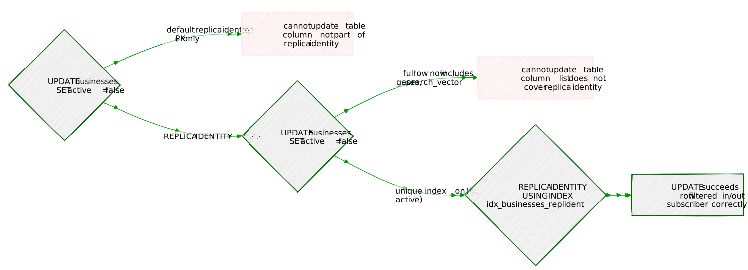
CREATE SUBSCRIPTION is PostgreSQL talking to PostgreSQL
— the wire format (pgoutput) is a compact binary protocol
meant for another PostgreSQL server to decode, not for a human or a
general-purpose client to read directly. Anything that wants to consume
the raw change stream — a custom sync tool, or (Exercise 6)
Debezium — talks the same underlying replication protocol, just with a
different output plugin and its own logic for what to do with each
change.
Not every downstream consumer of Portsmith’s data wants a full
PostgreSQL database, though. Suppose IT also wants to keep a search
index warm, or fire an internal Slack alert whenever a jobs
row lands in failed — neither of those is “spin up another
Postgres and CREATE SUBSCRIPTION,” it’s “run a lightweight
process that reacts to each change.” This exercise builds the simplest
version of exactly that: reading the change stream directly, with
nothing between it and the WAL.
5.1 — A second, independent slot
-- in portsmith
SELECT pg_create_logical_replication_slot('demo_test_decoding', 'test_decoding');test_decoding ships with core PostgreSQL and produces
human-readable text instead of pgoutput’s binary format —
the right choice for reading the stream directly rather than
feeding it to another PostgreSQL instance. This slot is entirely
independent of portsmith_sub — the same WAL, decoded twice,
for two different consumers.
5.2 — psycopg has no high-level replication API
Unlike psycopg2, which ships a purpose-built
LogicalReplicationConnection, psycopg (v3,
used throughout this book) doesn’t wrap the replication protocol at all.
It’s still fully reachable, though, through the same low-level
pq connection object every higher-level psycopg call is
eventually built on:
#!/usr/bin/env python3.12
# ch18_replication_stream.py — consume a logical replication slot directly
import struct
import time
import psycopg
SLOT_NAME = "demo_test_decoding"
conn = psycopg.connect("dbname=portsmith replication=database", autocommit=True)
pgconn = conn.pgconn
pgconn.exec_(f"START_REPLICATION SLOT {SLOT_NAME} LOGICAL 0/0".encode())
while True:
data = pgconn.get_copy_data(1) # 1 = non-blocking
if data[0] == 0:
pgconn.consume_input()
time.sleep(0.1)
continue
payload = bytes(data[1])
msg_type = payload[0:1]
if msg_type == b"w": # XLogData: an actual decoded change
wal_start = struct.unpack("!Q", payload[1:9])[0]
body = payload[25:].decode("utf-8", errors="replace")
print(f"[{wal_start:X}] {body}")
elif msg_type == b"k": # Primary keepalive
wal_end, _send_time, reply_requested = struct.unpack("!QQb", payload[1:18])
if reply_requested:
# must reply, or the server eventually decides this client is dead
now = int(time.time() * 1_000_000) - 946_684_800_000_000
pgconn.put_copy_data(b"r" + struct.pack("!QQQQb", wal_end, wal_end, wal_end, now, 0))START_REPLICATION puts the connection into COPY
BOTH mode — the same bidirectional streaming protocol
PostgreSQL’s own physical replication uses, just carrying decoded
logical changes instead of raw WAL bytes. Two message types arrive:
w (an actual change, XLogData) and
k (a keepalive the server sends periodically, which must be
acknowledged with a standby status update — skip that, and the server
eventually assumes the client has died and closes the connection). Full
script: data/ch18_replication_stream.py.
5.3 — Running it
python ch18_replication_stream.py --seconds 12While it runs, from another session:
INSERT INTO jobs (job_type, payload) VALUES ('demo_test', '{"note":"replication stream test"}');
UPDATE businesses SET employee_count = 10 WHERE id = 1;Real output:
[C6B57B98] table public.jobs: INSERT: id[bigint]:49 job_type[text]:'demo_test' payload[jsonb]:'{"note": "replication stream test"}' status[job_status]:'queued' priority[smallint]:5 ...
[C6B5A530] table public.businesses: UPDATE: id[integer]:1 name[text]:'The Gilded Clam' ... geom[geometry]:'0101000020E6100000FA7E6ABC7493FCBF9A99999999594940' employee_count[positive_integer]:'10' search_vector[tsvector]:'''clam'':3 ''gild'':2 ...' active[boolean]:trueNotice geom and search_vector are both
present here — columns portsmith_pub never publishes at
all. That’s the real distinction to take away: the WAL always
contains the whole row; a publication’s column list is a filter applied
on top of it, not something baked into what gets written to WAL in the
first place. A slot with no column list restriction, like this
one, sees everything; portsmith_sub, tied to
portsmith_pub, only ever sees what that publication chose
to expose.
Everything Exercise 5 hand-rolled — a replication slot, a decoding plugin, a loop reading changes and acknowledging keepalives — is exactly what Debezium’s PostgreSQL connector does, running as a Kafka Connect worker instead of a standalone script:
pgoutput (or the older
decoderbufs/wal2json plugins in older setups)
— structurally identical to portsmith_sub.portsmith.public.businesses,
portsmith.public.jobs — each message a JSON or Avro
envelope carrying the operation type (create,
update, delete, or read for the
initial snapshot), the row’s before-and-after image, and source metadata
(LSN, transaction ID, commit timestamp) — the same fields Exercise 5’s
raw XLogData messages carried, structured for machine
consumption instead of printed as text.confirmed_flush_lsn in Exercise 3’s
pg_replication_slots — Debezium periodically commits how
far it’s gotten, so a restart resumes from the right point in the WAL
instead of replaying everything or losing changes.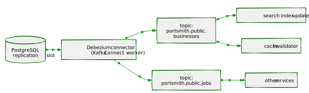
This is deliberately a discussion, not a hands-on exercise — a real
Debezium deployment needs Zookeeper (or KRaft), a Kafka broker, a Kafka
Connect worker, and the Debezium connector JARs, a multi-container stack
disproportionate to stand up for one exercise. What’s worth taking away
is that there’s no new mechanism to learn: Debezium is Exercise 5’s
script, hardened and made distributed, reading the exact same kind of
slot this chapter already created and drained by hand. Typical uses lean
on that continuous stream directly: keeping a search index or cache in
sync with PostgreSQL without a batch job’s inherent lag, or feeding a
businesses/jobs change feed into other
services in an event-driven architecture — the outbox
pattern, notably, uses exactly this to publish domain events
reliably, by writing them as ordinary rows in a transaction and letting
CDC carry them out instead of risking a dual-write to both a database
and a message queue.
| Concept | What it does |
|---|---|
wal_level = logical |
Required for any logical decoding — needs a restart, like
shared_preload_libraries |
CREATE PUBLICATION ... FOR TABLE t (cols) WHERE (expr) |
Scopes what’s streamed by table, column, and row |
| Replication slot | A durable bookmark retaining WAL for one consumer — exists independently of any subscription |
pg_create_subscription / REPLICATION
attribute |
Two separate gates: creating the local subscription object vs. opening a replication connection |
| Same-instance pub/sub deadlock | CREATE SUBSCRIPTION’s default
create_slot=true can wait on its own open transaction when
publisher and subscriber share an instance — pre-create the slot
instead |
pg_replication_slots /
pg_stat_replication |
Slot state and live lag — the detail columns of the latter need
pg_monitor |
ALTER SUBSCRIPTION ... REFRESH PUBLICATION |
Reconciles which tables are tracked — does not retroactively resync a changed column list or row filter on an already-synced table |
REPLICA IDENTITY USING INDEX |
The precise fix for filtering on a non-key column — wide enough to cover the filter, no wider than the publication’s own column list |
Raw replication protocol
(pgconn.get_copy_data/put_copy_data) |
What CREATE SUBSCRIPTION, Exercise 5’s script, and
Debezium all ultimately speak underneath |
| Debezium | The same slot/decode/apply loop, made distributed and production-grade, one Kafka topic per table |
The key design insight from this chapter is that a
replication slot is the one durable object underneath everything else —
CREATE SUBSCRIPTION, a hand-rolled psycopg script, and
Debezium are three different consumers of the exact same primitive,
differing only in what decodes the WAL and what happens to the output.
Understanding the slot is understanding the whole chapter; everything
else is a client.
Going further: Chapter 19’s pg_cron is the natural
next tool for operationalizing what this chapter demonstrated by hand —
a scheduled job that checks pg_replication_slots for a slot
whose confirmed_flush_lsn hasn’t advanced in too long (a
stuck or abandoned consumer, quietly retaining WAL) and pages someone
before disk fills up, the same shape of unattended, recurring
maintenance task Chapter 17’s own “going further” note imagined for
aging partition exports.
pg_cron: Scheduled Jobs Inside PostgreSQLA cron job that lives outside the database has to be told, from scratch, how to reach it. A cron job that lives inside the database is already there.
By this point in the book, Portsmith has quietly accumulated three
things that all need to happen on a schedule, and right now every one of
them depends on a person remembering to do it. Chapter 9’s
mv_sensor_daily — the rollup the public works dashboard
reads sensor trends from — only reflects reality as recently as whoever
last ran CALL refresh_and_log(...) by hand thought to run
it. Chapter 3’s permit-processing workers occasionally crash mid-job
without releasing what they were holding, and until someone remembers to
re-run ch03_reclaim.py, that permit just sits
in_progress forever, with no error, and no worker aware
it’s supposed to try again. And Chapter 17’s
businesses_archive, living quietly in
portsmith_legacy, gets so little ordinary traffic that
autovacuum’s usual change-percentage triggers rarely fire on it — its
planner statistics can go stale for months with nothing to notice.
None of these are hypothetical. The specific version of this that
actually happened while building this chapter’s demo data: a stalled
in_progress permit sat unprocessed for over half an hour
before anything caught it, because nothing was watching — exactly the
failure mode Exercise 4 reproduces on purpose. The pattern behind all
three is the same one every real system eventually hits: recurring
maintenance that depends on a human’s memory degrades quietly, not
loudly, and “someone should really schedule that” has a way of staying a
to-do item for months.
The traditional fix is an external scheduler — OS-level
cron, a workflow tool, or a sidecar container — that wakes
up on its own timeline and connects in from outside.
pg_cron takes a different position: it
runs inside PostgreSQL, as a background process the postmaster
manages like any other, reading its schedule from an ordinary table
(cron.job) and writing its history to another
(cron.job_run_details). Scheduling Portsmith’s daily
refresh, its stalled-job sweep, and the archive database’s
ANALYZE all become a SELECT, not three
separate deployments to babysit.
That proximity is also exactly where this chapter’s real gotchas come
from: a job that “lives inside PostgreSQL” doesn’t skip the parts of
PostgreSQL that would normally apply to any other client connecting in —
it still needs a role, that role still needs privileges, and if a
password is required to connect as that role, pg_cron’s own
connection needs one too, from somewhere.
Three of Portsmith’s own real, already-built pieces become this chapter’s scheduled jobs — nothing new needs inventing, only automating:
| Object | Source | Purpose |
|---|---|---|
refresh_and_log(regclass) |
Chapter 9 | Keeps the public works dashboard’s mv_sensor_daily
rollup from going stale, without anyone running it by hand |
jobs / dead_letter_jobs |
Chapter 3 | The permit queue itself — where a crashed worker’s abandoned,
still-in_progress job would otherwise sit forever |
sweep_stalled_jobs() |
(new) | SQL port of ch03_reclaim.py’s stalled-job logic, so the
sweep can run unattended instead of by hand |
guarded_demo_task() |
(new) | Teaching-only procedure demonstrating advisory-lock overlap guards |
businesses_archive |
Chapter 17, portsmith_legacy |
The rarely-touched archive table whose planner statistics need a
scheduled ANALYZE, since ordinary traffic won’t trigger
one |
By the end of this chapter you will be able to:
pg_cron, schedule a job, and know exactly which
two real walls a first attempt hits before a job actually runs.cron.job and cron.job_run_details
correctly — including a sorting mistake that’s easy to make and easy to
miss.pg_cron already protects you
from around overlapping runs, and what it doesn’t — and use an advisory
lock for the part it doesn’t.pg_cron itself runs in.cron.job_run_details as a first-class thing to alert
on.sudo apt install postgresql-16-cron# postgresql.conf — shared across this chapter and the next two
shared_preload_libraries = 'pg_cron,pg_stat_statements,auto_explain'
cron.database_name = 'portsmith'sudo systemctl restart postgresql-- as postgres
CREATE EXTENSION pg_cron;cron.database_name matters beyond just naming a
database: it’s where pg_cron’s own launcher process runs
and where cron.job / cron.job_run_details live
— Exercise 5’s whole point is scheduling a job that runs somewhere
other than this one database.
pg_cron and Scheduling an Hourly
Refresh1.1 — Schedule it
Chapter 9’s refresh_and_log() procedure already does
everything an hourly refresh needs — pg_cron’s job is just
to call it on a schedule instead of leaving it to whoever on the public
works team remembers to run it that day:
SELECT cron.schedule('refresh-mv-sensor-daily', '0 * * * *',
$$CALL refresh_and_log('mv_sensor_daily')$$);ERROR: permission denied for schema cronCreating the extension doesn’t hand every role access to its schema —
familiar territory by now (Chapter 17’s
GRANT USAGE ON FOREIGN DATA WRAPPER, Chapter 10’s
api schema):
-- as postgres
GRANT USAGE ON SCHEMA cron TO chris;
GRANT SELECT ON cron.job, cron.job_run_details TO chris;
GRANT EXECUTE ON FUNCTION cron.schedule(text,text,text) TO chris;A natural instinct is to grant every cron.* function
chris might need, all at once, in one -c call — which
surfaces a real trap:
ERROR: function cron.schedule_in_database(text, text, text, text) does not existThat one function’s signature didn’t match this pg_cron
version — and because multiple ;-separated statements sent
as one -c string run as a single implicit transaction,
the entire batch rolled back, including the
GRANT USAGE ON SCHEMA that had appeared to succeed a moment
before. The fix is both a narrower ask and a more robust one — grant
every function in the schema by wildcard instead of enumerating
signatures you’d have to get exactly right:
-- as postgres, in one clean batch
GRANT USAGE ON SCHEMA cron TO chris;
GRANT SELECT ON cron.job, cron.job_run_details TO chris;
GRANT EXECUTE ON ALL FUNCTIONS IN SCHEMA cron TO chris;SELECT cron.schedule('refresh-mv-sensor-daily', '* * * * *', -- every minute, to verify quickly
$$CALL refresh_and_log('mv_sensor_daily')$$); schedule
----------
21.2 — It “succeeds,” but nothing actually runs
SELECT jobid, status, return_message FROM cron.job_run_details WHERE jobid = 2; jobid | status | return_message
-------+--------+-------------------
2 | failed | connection failed
2 | failed | connection failedNo further detail, and nothing in the PostgreSQL log even shows a
rejected authentication attempt — the connection is failing before it
gets that far. The reason: pg_cron’s launcher runs as the
postgres OS user, and to actually execute
a job it opens its own new connection to the target database,
authenticating as whichever role owns the job (chris).
That’s a different OS user than the one chris’s own
interactive psql sessions run as, and — same wall Chapter
17 hit with postgres_fdw — a non-superuser connecting this
way needs a real password, which nothing here has supplied yet. The fix
is the standard one for a background process needing a password it can’t
be prompted for: a .pgpass file, owned by the OS user
running PostgreSQL:
sudo -u postgres bash -c 'echo "localhost:5432:portsmith:chris:fdw-demo-password" >> ~/.pgpass && chmod 600 ~/.pgpass'SELECT jobid, status, return_message, start_time, end_time FROM cron.job_run_details WHERE jobid = 2 ORDER BY runid DESC LIMIT 2; jobid | status | return_message | start_time | end_time
-------+-----------+-----------------+-------------------------------+-------------------------------
2 | succeeded | CALL | 2026-08-09 23:27:00.015674-04 | 2026-08-09 23:27:02.030591-04
2 | succeeded | CALL | 2026-08-09 23:26:00.018446-04 | 2026-08-09 23:26:02.405988-04Real, unattended, one-minute-apart refreshes, each taking about two seconds. With it proven working, dial back to the real cadence:
SELECT cron.alter_job(2, schedule := '0 * * * *');
cron.job and
cron.job_run_detailsSELECT jobid, jobname, schedule, command, active FROM cron.job; jobid | jobname | schedule | command
-------+--------------------------+------------+-------------------------------------------
2 | refresh-mv-sensor-daily | 0 * * * * | CALL refresh_and_log('mv_sensor_daily')cron.job_run_details is the run history — and it has a
sorting trap worth knowing before it costs debugging time. The failed
runs from Exercise 1.2 never got a start_time at all (the
connection never opened far enough to set one):
SELECT jobid, status, start_time FROM cron.job_run_details ORDER BY start_time DESC LIMIT 5; jobid | status | start_time
-------+--------+--------------------------------
2 | failed |
2 | failed |
2 | failed |
2 | succeeded | 2026-08-09 23:27:00.015674-04
2 | succeeded | 2026-08-09 23:26:00.018446-04ORDER BY ... DESC sorts NULL as the
largest possible value by default — so the oldest failures, the
ones with no timestamp at all, appear to be “first” ahead of genuinely
recent successes. Anyone scanning this for “what happened most recently”
and trusting the sort order would read yesterday’s failures as more
current than this minute’s successes. The fix is either an explicit
NULLS LAST, or sorting by runid (monotonic,
never null) instead:
SELECT jobid, status, start_time FROM cron.job_run_details ORDER BY start_time DESC NULLS LAST LIMIT 5; jobid | status | start_time
-------+-----------+--------------------------------
2 | succeeded | 2026-08-09 23:27:00.015674-04
2 | succeeded | 2026-08-09 23:26:00.018446-04
2 | failed |
2 | failed |
2 | failed |pg_cron Already Does, and What
It Doesn’t3.1 — A deliberately slow job
CREATE OR REPLACE PROCEDURE guarded_demo_task(delay_seconds int DEFAULT 0)
LANGUAGE plpgsql AS $$
BEGIN
IF NOT pg_try_advisory_lock(hashtext('guarded_demo_task')) THEN
RAISE NOTICE 'already running, skipping this run';
RETURN;
END IF;
PERFORM pg_sleep(delay_seconds);
RAISE NOTICE 'did the work';
PERFORM pg_advisory_unlock(hashtext('guarded_demo_task'));
END;
$$;
SELECT cron.schedule('guarded-demo', '* * * * *', $$CALL guarded_demo_task(75)$$);A 75-second job on a 60-second schedule guarantees overlap — the
question is what pg_cron actually does about it.
3.2 — pg_cron already refuses to double-run the
same job
LOG: cron job 3 starting: CALL guarded_demo_task(75) -- 23:28:00
LOG: cron job 3 COMMAND completed: CALL -- 23:29:15
LOG: cron job 3 starting: CALL guarded_demo_task(75) -- 23:29:15, immediately afterThere’s no log line for a job 3 start at 23:29:00 at all —
pg_cron noticed the previous run of this exact
jobid was still going and simply didn’t launch a second one
for that tick. It doesn’t queue the missed tick either: the next run
starts the instant a slot frees, at 23:29:15, not at the next minute
boundary. Left running long enough, the schedule drifts further from the
clock with every overlap, a real and worth-knowing side effect on its
own.
3.3 — What that protection doesn’t cover
pg_cron’s serialization is scoped to one
jobid. It says nothing about the same underlying task being
triggered a second way — a different job entry calling the same
procedure, or a human running it by hand. While job 3 was mid-run:
CALL guarded_demo_task(0); -- from an ordinary psql session, not cron at allNOTICE: already running, skipping this run
CALLThis is what the advisory lock actually earns its keep for —
not the same-jobid case pg_cron already
handles, but any other path that might reach the same resource
concurrently. The lock is keyed on the resource
(guarded_demo_task, or in a real refresh job’s case,
probably the matview’s name), not on the job — which is exactly what
lets it catch a case pg_cron’s own per-job serialization
structurally can’t.
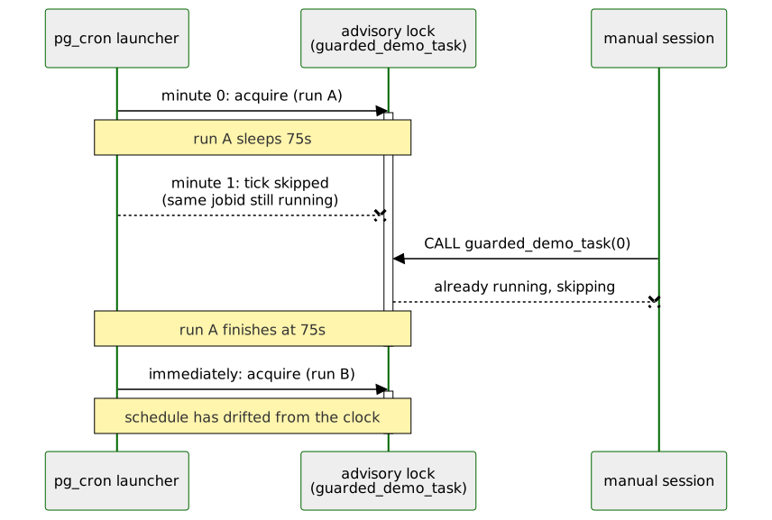
SELECT cron.unschedule('guarded-demo');Chapter 3 built ch03_reclaim.py to requeue stalled jobs
and dead-letter the ones that exhausted their retries — run by hand, or
“on a schedule (see Chapter 19),” per its own docstring at the time.
That schedule is this exercise: the same logic, as a SQL function
pg_cron can call directly, no external process required.
Practically, this is the fix for the exact failure mode described in the
Background: a permit worker crashes, its job is left
in_progress with a heartbeat that stops updating, and
without this sweep running on its own, nothing ever notices until the
applicant calls asking why their permit hasn’t moved in three weeks.
4.1 — Port the script’s logic to SQL
CREATE OR REPLACE FUNCTION sweep_stalled_jobs(p_timeout interval DEFAULT interval '30 minutes')
RETURNS TABLE(requeued int, dead_lettered int)
LANGUAGE plpgsql AS $$
DECLARE
r RECORD;
v_requeued int := 0;
v_dead_lettered int := 0;
v_error text;
BEGIN
FOR r IN
SELECT id, job_type, attempts, max_attempts, claimed_by, heartbeat_at
FROM jobs
WHERE status = 'in_progress' AND heartbeat_at < now() - p_timeout
ORDER BY id
LOOP
v_error := format('stalled: no heartbeat since %s (last claimed by %s)', r.heartbeat_at, r.claimed_by);
IF r.attempts >= r.max_attempts THEN
WITH failed AS (
DELETE FROM jobs WHERE id = r.id
RETURNING id, job_type, payload, priority, attempts, max_attempts, created_at
)
INSERT INTO dead_letter_jobs (id, job_type, payload, priority, attempts, max_attempts, created_at, last_error)
SELECT id, job_type, payload, priority, attempts, max_attempts, created_at, v_error FROM failed;
v_dead_lettered := v_dead_lettered + 1;
ELSE
UPDATE jobs SET status = 'queued', claimed_at = NULL, claimed_by = NULL,
heartbeat_at = NULL, last_error = v_error
WHERE id = r.id;
v_requeued := v_requeued + 1;
END IF;
END LOOP;
RETURN QUERY SELECT v_requeued, v_dead_lettered;
END;
$$;4.2 — Prove both branches work
INSERT INTO jobs (job_type, payload, status, priority, attempts, max_attempts, claimed_at, claimed_by, heartbeat_at)
VALUES ('demo_stall_requeue', '{}', 'in_progress', 5, 1, 3, now() - interval '40 minutes', 'worker-demo', now() - interval '35 minutes'),
('demo_stall_deadletter', '{}', 'in_progress', 5, 3, 3, now() - interval '40 minutes', 'worker-demo', now() - interval '35 minutes');
SELECT * FROM sweep_stalled_jobs(); requeued | dead_lettered
----------+----------------
1 | 1SELECT id, status FROM jobs WHERE job_type = 'demo_stall_requeue';
SELECT id, last_error FROM dead_letter_jobs WHERE job_type = 'demo_stall_deadletter'; id | status
----+-----------
51 | queued
id | last_error
----+-------------------------------------------------------------------------------------------
52 | stalled: no heartbeat since 2026-08-09 21:47:19.767251-04 (last claimed by worker-demo)Exactly the two outcomes ch03_reclaim.py produced by
hand — attempts remaining gets requeued, retries exhausted gets
dead-lettered, with a descriptive last_error either
way.
4.3 — Schedule it
SELECT cron.schedule('sweep-stalled-jobs', '*/5 * * * *', $$SELECT sweep_stalled_jobs()$$);Verified live with a fresh stalled job and a one-minute test schedule
before settling on every five minutes: job_run_details
showed status: succeeded,
return_message: 1 row, and the planted job’s
status really did flip back to queued — the
scheduled path produces the same result as the manual call in 4.2, just
unattended.
cron.schedule_in_database()cron.database_name = 'portsmith' means
pg_cron’s launcher itself lives there — every job scheduled
with plain cron.schedule() runs against
portsmith by definition.
cron.schedule_in_database() is the escape hatch: a job that
runs against a different database entirely, using the
same underlying launcher. businesses_archive is exactly the
kind of table this matters for: since Chapter 17, almost nothing writes
to it directly, so it rarely crosses autovacuum’s change-percentage
threshold for an automatic ANALYZE on its own — left alone,
its planner statistics just quietly drift out of date.
SELECT cron.schedule_in_database('legacy-analyze', '0 4 * * *',
'ANALYZE businesses_archive;', 'portsmith_legacy');Verified against portsmith_legacy — Chapter 17’s second
database — by checking the one thing ANALYZE actually
changes:
-- in portsmith_legacy, before
SELECT last_analyze FROM pg_stat_user_tables WHERE relname = 'businesses_archive'; last_analyze
---------------
(null)-- in portsmith, briefly rescheduled to every 2 minutes to verify quickly
SELECT cron.alter_job((SELECT jobid FROM cron.job WHERE jobname = 'legacy-analyze'), schedule := '*/2 * * * *');-- in portsmith_legacy, ~2 minutes later
SELECT last_analyze FROM pg_stat_user_tables WHERE relname = 'businesses_archive'; last_analyze
-------------------------------
2026-08-09 23:28:00.039363-04A real, verified timestamp — pg_cron’s single launcher
process, still physically running inside portsmith, reached
across and executed SQL against a completely different database. Reset
to a realistic once-daily cadence once proven:
SELECT cron.alter_job((SELECT jobid FROM cron.job WHERE jobname = 'legacy-analyze'), schedule := '0 4 * * *');6.1 — cron.alter_job() and
cron.unschedule()
Both already used for real, twice each, in Exercises 1, 3, and 5 —
alter_job to change a schedule without dropping and
recreating the job (its history in job_run_details stays
intact, keyed by the same jobid), unschedule
to remove one outright.
6.2 — A job that genuinely fails
SELECT cron.schedule('broken-demo-job', '* * * * *', 'SELECT * FROM this_table_does_not_exist;');SELECT status, return_message FROM cron.job_run_details ORDER BY runid DESC LIMIT 1; status | return_message
--------+--------------------------------------------------------------
failed | ERROR: relation "this_table_does_not_exist" does not exist
| LINE 1: SELECT * FROM this_table_does_not_exist;
| ^The real error text, captured and stored — pg_cron
doesn’t swallow failures, it logs exactly what PostgreSQL would have
said to an interactive session running the same statement.
SELECT cron.unschedule('broken-demo-job');6.3 — The monitoring query this chapter has been building toward
SELECT jobid, status, return_message, start_time
FROM cron.job_run_details
WHERE status = 'failed'
ORDER BY start_time DESC NULLS LAST
LIMIT 10;The same NULLS LAST fix from Exercise 2, now doing real
work: a recurring check for exactly this query, scheduled itself (or
wired into existing alerting), is the difference between a scheduled job
failing silently for weeks and someone finding out the same day.
| Concept | What it does |
|---|---|
cron.schedule(name, schedule, command) |
Registers a job — needs USAGE on schema
cron plus EXECUTE on its functions |
.pgpass for the PostgreSQL OS user |
Required for pg_cron’s background connection to
authenticate as a non-superuser job owner |
cron.job / cron.job_run_details |
Schedule and run history — sort job_run_details by
runid or with NULLS LAST, never a bare
start_time DESC |
Same-jobid overlap |
Already prevented by pg_cron itself — a missed tick
isn’t queued, the next run starts immediately once a slot frees |
| Cross-path overlap (different jobs, or a manual call) | Not covered by pg_cron — needs its own
pg_try_advisory_lock, keyed on the resource, not the
job |
cron.schedule_in_database(name, schedule, command, database) |
Runs against a database other than
cron.database_name |
cron.alter_job() / cron.unschedule() |
Modify a job in place (history preserved) or remove it entirely |
cron.job_run_details.status = 'failed' |
A real, monitorable signal — the same shape of query worth alerting on, not just reading by hand |
The key design insight from this chapter is that
pg_cron gives you exactly one guarantee for free — a job
won’t overlap with its own previous run — and that guarantee is narrower
than it first sounds. Everything else a production scheduler needs
(locking scoped to the actual shared resource, credentials for the
connection it opens on your behalf, monitoring that actually gets read)
is the same responsibility it would be with any external scheduler, just
moved inside a table instead of a config file.
Going further: Chapter 20’s pg_stat_statements and
auto_explain — already sharing this chapter’s
shared_preload_libraries line — turn the same kind of “what
actually happened” question this chapter asked of
cron.job_run_details onto query performance instead of
scheduled jobs. And Exercise 4’s sweep_stalled_jobs() is
worth pairing with Chapter 18’s own “going further” note: a second
pg_cron job that watches pg_replication_slots
for a slot whose confirmed_flush_lsn has stopped advancing
is the exact same “scheduled health check” shape applied to replication
instead of the job queue.
pg_stat_statements and Query Performance“It’s slow” is a feeling. “This queryid has a mean execution time of 440ms across 964,800 rows touched, up from 47ms last week” is a fact — and only one of those is actionable.
Every chapter so far has looked at PostgreSQL from the perspective of what it can store and how to query it correctly. This chapter asks a different question of the exact same database: not is this query right, but is this query fast, and if not, why not, and how would you know before a user told you. Three tools, working together:
pg_stat_statements — every statement
PostgreSQL runs, normalized (literal values replaced with
$1, $2, …) and aggregated: call count, total
time, mean time, rows, buffers. The answer to “what’s actually slow, in
aggregate, right now.”EXPLAIN (ANALYZE, BUFFERS) — the
answer to “why,” for one specific query: the plan PostgreSQL actually
chose, with real timing and real I/O counts, not just the planner’s
estimate.auto_explain — the same
EXPLAIN output, captured automatically for any query slower
than a threshold you set, without needing to already suspect which query
to go looking for.Chapter 19 treated cron.job_run_details as a first-class
thing to monitor rather than just read once by hand. This chapter
applies the same discipline to query performance: not a one-time
diagnosis, but an ongoing signal worth checking after every deploy.
This chapter intentionally introduces the three classic shapes of slow query against tables already built by earlier chapters — nothing new seeded, everything real:
| Problem | Where |
|---|---|
| An implicit cast defeating an index | businesses.id (Chapter 1) |
| A missing index on a large table | sensor_readings (Chapter 8, 9.6M rows) |
| A plan regression after a schema change | The same sensor_readings index, deliberately dropped
and restored |
By the end of this chapter you will be able to:
EXPLAIN (ANALYZE, BUFFERS) plan node by
node.auto_explain to capture slow-query plans without
needing to already know which query to chase.pg_stat_statements and auto_explain were
already added to shared_preload_libraries alongside
pg_cron back in Chapter 19’s setup, and
pg_stat_statements was created as an extension at the same
time:
-- as postgres, in portsmith — already done in Chapter 19's setup
CREATE EXTENSION pg_stat_statements;Two functions this chapter needs are both revoked from
PUBLIC by default — worth granting up front rather than
mid-exercise:
-- as postgres
GRANT EXECUTE ON FUNCTION pg_stat_statements_reset(oid, oid, bigint) TO chris;
GRANT EXECUTE ON FUNCTION pg_reload_conf() TO chris;The first attempt at the reset grant is worth knowing about even
though it’s avoided here: pg_stat_statements_reset() — no
arguments — doesn’t exist in current versions; the real signature takes
three optional filter arguments (userid, dbid,
queryid, all defaulting to 0, meaning “reset
everything”). \df pg_stat_statements_reset is the fast way
to check a signature before writing a GRANT for it, instead
of guessing.
SELECT pg_stat_statements_reset();A representative mix of real queries against this book’s data — some run often and cheap, one run rarely but expensive:
SELECT query, calls, round(total_exec_time::numeric, 2) AS total_ms,
round(mean_exec_time::numeric, 3) AS mean_ms, rows
FROM pg_stat_statements
ORDER BY total_exec_time DESC
LIMIT 10; query | calls | total_ms | mean_ms | rows
------------------------------------------------------------------------------------------------+-------+----------+---------+-------
SELECT count(*) FROM sensor_readings WHERE sensor_type = $1 | 2 | 879.08 | 439.541 | 2
SELECT * FROM businesses WHERE id = $1 | 30 | 160.14 | 5.338 | 30
SELECT * FROM sensor_readings WHERE sensor_id = $1 AND recorded_at >= $2 AND recorded_at < $3 | 15 | 55.18 | 3.678 | 23520
SELECT * FROM businesses WHERE details @> $1 | 10 | 46.31 | 4.631 | 150
SELECT id FROM jobs WHERE status = $1 ORDER BY priority, created_at LIMIT $2 FOR UPDATE SKIP LOCKED | 25 | 2.26 | 0.090 | 25Two real lessons sitting side by side. First, literal values are
normalized away ($1, $2) — every call to “look
up one business by id” collapses into a single row here regardless of
which id, which is exactly what makes aggregation meaningful
instead of one row per unique query text. Second, and the actual point
of ranking by total_exec_time rather than
mean_exec_time: a query called only twice
(an unindexed count(*) over 9.6 million rows) costs more in
aggregate than a well-indexed lookup called thirty
times. Frequency and per-call cost are independent axes, and a
rare expensive query hiding behind a wall of cheap frequent ones is
precisely what this view is for catching.
EXPLAIN (ANALYZE, BUFFERS, FORMAT TEXT)
SELECT * FROM sensor_readings WHERE sensor_id = 5; Gather (cost=1000.00..151794.26 rows=97046 width=42) (actual time=12.772..300.728 rows=96480 loops=1)
Workers Planned: 2
Workers Launched: 2
Buffers: shared hit=1812 read=88823
-> Parallel Append (cost=0.00..141089.66 rows=40436 width=42) (actual time=13.683..273.244 rows=32160 loops=3)
Buffers: shared hit=1812 read=88823
-> Parallel Seq Scan on sensor_readings_2024_03 sensor_readings_2 (cost=0.00..13034.00 rows=3608 width=42) (actual time=14.335..84.003 rows=8928 loops=1)
Filter: (sensor_id = 5)
Rows Removed by Filter: 883872
Buffers: shared hit=129 read=8255
... (one Parallel Seq Scan per partition)
Planning Time: 1.980 ms
Execution Time: 338.496 msNode by node, outside in:
| Node | Meaning |
|---|---|
Gather |
The parallel query’s top: collects rows from worker processes back into one stream |
Workers Planned / Launched |
How many parallel workers PostgreSQL asked for vs. actually got — a
mismatch here would itself be worth investigating
(max_parallel_workers exhausted) |
Parallel Append |
Chapter 8’s partitioning at work: each partition scanned independently, results appended |
Parallel Seq Scan on sensor_readings_2024_03 |
One partition, scanned start to finish — no index used |
Filter: (sensor_id = 5) |
The condition applied after reading each row — the tell that no index narrowed things down first |
Rows Removed by Filter: 883872 |
Nearly 884,000 rows read and discarded, in this partition alone, to find the ~9,000 that matched |
Buffers: shared hit=... read=... |
hit = found in PostgreSQL’s own buffer cache;
read = a real disk read — read=88823 here
means the bulk of this query’s cost is genuine I/O, not CPU |
Execution Time: 338.496 ms |
The number that actually matters to whoever’s waiting on this query |
ANALYZE runs the query for real and reports actual
timing and row counts alongside the planner’s original estimates;
BUFFERS adds the I/O accounting. Without both,
EXPLAIN alone only shows what PostgreSQL expected,
not what happened.
EXPLAIN (ANALYZE, BUFFERS) SELECT * FROM businesses WHERE id = 5; Index Scan using idx_businesses_replident on businesses (cost=0.14..8.16 rows=1 width=783) (actual time=0.191..0.192 rows=1 loops=1)
Index Cond: (id = 5)
Buffers: shared read=2Index Cond, two buffer reads — exactly what a
primary-key lookup should look like. Now the same lookup, with a value
typed as numeric instead of integer — the kind
of thing a client library can do silently (a JSON-decoded number, a
Python Decimal, an ORM’s default type mapping for a
“generic number” field):
EXPLAIN (ANALYZE, BUFFERS) SELECT * FROM businesses WHERE id = 5::numeric; Seq Scan on businesses (cost=0.00..8.73 rows=1 width=783) (actual time=0.011..0.313 rows=1 loops=1)
Filter: ((id)::numeric = '5'::numeric)
Rows Removed by Filter: 47
Buffers: shared hit=1 read=7Filter, not Index Cond — PostgreSQL has
wrapped the column in a cast ((id)::numeric) to
make the comparison type-consistent, and a plain btree index on
id (built on integer values) can’t be used to
satisfy a condition on id::numeric. On a 49-row table the
wall-clock difference is invisible — both finish in under half a
millisecond, buried in connection overhead. The plan shape is identical,
though, to Exercise 4’s sensor_id lookup before it had the
right index: exactly this bug against a multi-million-row table is how a
sub-millisecond primary-key lookup silently becomes a 300ms sequential
scan, and nothing about the query’s result looks wrong — it
just gets slower, quietly, as the table grows.
The fix is whichever side of the comparison is easiest to control:
cast the parameter instead of leaving the column to be cast
(id = $1::integer at the application layer), or, if the
value’s type is genuinely outside your control, an expression index on
(id::numeric) — though matching the parameter’s type going
in is almost always the better fix.
4.1 — The baseline
sensor_readings has no index on sensor_id
at all — every lookup by sensor scans every partition:
EXPLAIN (ANALYZE, BUFFERS) SELECT * FROM sensor_readings WHERE sensor_id = 5; Gather (actual time=12.772..300.728 rows=96480 loops=1)
-> Parallel Append ...
(12 Parallel Seq Scans, one per partition)
Execution Time: 338.496 ms4.2 — The obvious fix helps less than expected
CREATE INDEX idx_sensor_readings_sensor_id ON sensor_readings (sensor_id);EXPLAIN (ANALYZE, BUFFERS) SELECT * FROM sensor_readings WHERE sensor_id = 5; Append (actual time=1.629..401.335 rows=96480 loops=1)
Buffers: shared hit=225 read=81071 written=35
-> Bitmap Heap Scan on sensor_readings_2024_02 ...
Buffers: shared hit=131 read=6907
-> Bitmap Index Scan on sensor_readings_2024_02_sensor_id_idx ...
Execution Time: 376.942 msSlower, not faster — a real, worth-understanding
result, not a mistake to paper over. Sensor 5 has 96,480 readings out of
9.6 million, roughly one row in 120, spread essentially evenly across
the whole table’s history — every month, every day, interleaved with
every other sensor’s readings. A Bitmap Heap Scan still
has to visit almost every 8KB heap page, because at that scatter,
virtually every page contains at least one matching row. The index made
the search for matching rows cheap
(Bitmap Index Scan) but did nothing about the
fetch cost, which dominates — and switching from a Parallel Seq
Scan to a plain Bitmap Heap Scan even gave up the free parallelism the
original plan had. An index is not automatically a win; it’s a trade
worth actually measuring.
4.3 — The query that was never realistic in the first place
Nobody actually asks for “all of sensor 5’s history, unbounded.” A real query narrows by time too — and Chapter 8’s partitioning already helps here, with no new index at all:
DROP INDEX idx_sensor_readings_sensor_id;
EXPLAIN (ANALYZE, BUFFERS)
SELECT * FROM sensor_readings
WHERE sensor_id = 5 AND recorded_at >= '2024-06-01' AND recorded_at < '2024-06-08'; Gather (actual time=0.301..35.504 rows=2016 loops=1)
-> Parallel Seq Scan on sensor_readings_2024_06 sensor_readings
Filter: (... AND sensor_id = 5)
Rows Removed by Filter: 287328
Execution Time: 35.671 msPartition pruning alone — only sensor_readings_2024_06
touched, not all twelve — already beats Exercise 4.2’s “fix.” The right
index closes the rest of the gap:
CREATE INDEX idx_sensor_readings_sensor_time ON sensor_readings (sensor_id, recorded_at);EXPLAIN (ANALYZE, BUFFERS)
SELECT * FROM sensor_readings
WHERE sensor_id = 5 AND recorded_at >= '2024-06-01' AND recorded_at < '2024-06-08'; Bitmap Heap Scan on sensor_readings_2024_06 sensor_readings (actual time=0.587..7.534 rows=2016 loops=1)
Recheck Cond: (sensor_id = 5 AND recorded_at >= ... AND recorded_at < ...)
Heap Blocks: exact=1697
Buffers: shared read=1708
-> Bitmap Index Scan on sensor_readings_2024_06_sensor_id_recorded_at_idx
Buffers: shared read=11
Execution Time: 7.878 ms7.9ms — roughly 4.5x faster than pruning alone, roughly 43x faster than the original unbounded query, and the honest conclusion of the whole exercise: the single-column index in 4.2 wasn’t wrong because indexes are bad, it was wrong because it didn’t match how the table is actually queried. A compound index over both the filter column and the range column, paired with a query shape that was already realistic, is what actually won.
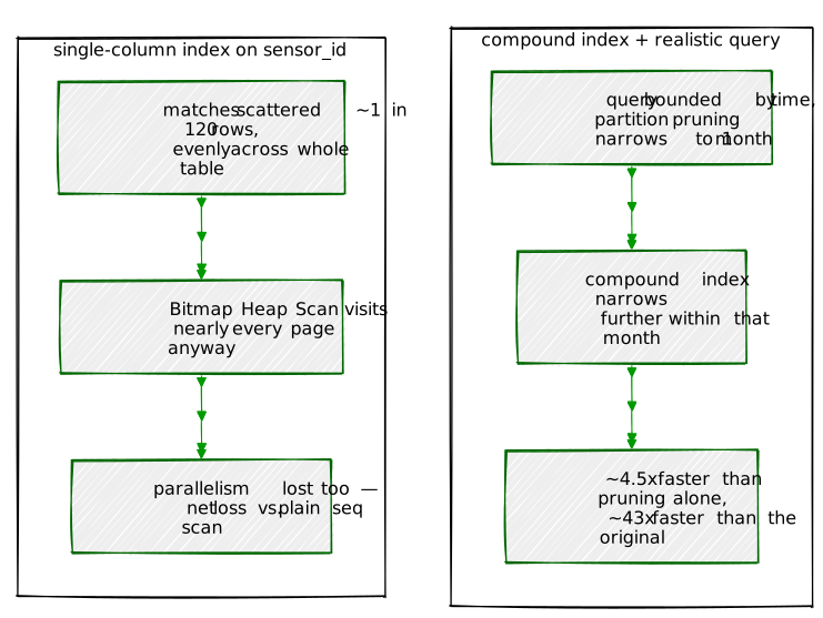
auto_explain: Catching Slow Queries Without Knowing to
Lookauto_explain was proven working back in Chapter 19’s
environment setup, logging every query at
log_min_duration = 0. That’s useful for a five-minute test
and useless in production — it would flood the log. A realistic
threshold, and turning it on requires nothing at the session level (it’s
already preloaded cluster-wide):
-- as postgres
ALTER SYSTEM SET auto_explain.log_min_duration = 200; -- millisecondsReloading config needs its own grant, same shape as
pg_stat_statements_reset() above:
GRANT EXECUTE ON FUNCTION pg_reload_conf() TO chris;SELECT pg_reload_conf();SELECT * FROM businesses WHERE id = 3; -- fast — should stay silent
SELECT count(*) FROM sensor_readings WHERE sensor_type = 'air_quality'; -- slow — should logThe fast lookup produces nothing in the log. The slow one:
LOG: duration: 374.630 ms plan:
Query Text: SELECT count(*) FROM sensor_readings WHERE sensor_type = 'air_quality';
Finalize Aggregate (actual time=367.286..374.621 rows=1 loops=1)
Buffers: shared hit=15377 read=75258
-> Gather (actual time=367.178..374.609 rows=3 loops=1)
Workers Planned: 2
Workers Launched: 2
-> Partial Aggregate (actual time=354.058..354.061 rows=1 loops=3)
-> Parallel Append (actual time=16.793..340.363 rows=321600 loops=3)Captured automatically, no application code changed, no prior
suspicion needed about which query would be the slow one — exactly
sensor_type doing what Exercise 1’s top-10 already flagged
as the single most expensive query in the whole workload, this time
caught by threshold instead of by manually going looking.
The point of watching query performance continuously rather than once: catching a regression the moment a deploy introduces it, not weeks later when someone complains. A minimal snapshot table and a real before/after comparison:
6.1 — Snapshot before a “deploy”
CREATE TABLE query_stats_snapshot (
snapshot_label TEXT,
snapshot_at TIMESTAMPTZ DEFAULT clock_timestamp(),
queryid BIGINT,
query TEXT,
calls BIGINT,
mean_exec_time DOUBLE PRECISION
);
SELECT pg_stat_statements_reset();
-- ... run representative traffic ...
INSERT INTO query_stats_snapshot (snapshot_label, queryid, query, calls, mean_exec_time)
SELECT 'before_deploy', queryid, query, calls, mean_exec_time
FROM pg_stat_statements
WHERE query LIKE 'SELECT * FROM sensor_readings WHERE sensor_id%';6.2 — Simulate the incident: a deploy accidentally drops the index
SELECT pg_stat_statements_reset();
DROP INDEX idx_sensor_readings_sensor_time; -- Exercise 4's fix, reverted "by accident"
-- ... same representative traffic again ...
INSERT INTO query_stats_snapshot (snapshot_label, queryid, query, calls, mean_exec_time)
SELECT 'after_deploy', queryid, query, calls, mean_exec_time
FROM pg_stat_statements
WHERE query LIKE 'SELECT * FROM sensor_readings WHERE sensor_id%';6.3 — Compare
SELECT b.mean_exec_time AS before_ms, a.mean_exec_time AS after_ms,
round((a.mean_exec_time / b.mean_exec_time)::numeric, 1) AS slowdown_factor
FROM query_stats_snapshot b
JOIN query_stats_snapshot a ON a.queryid = b.queryid AND a.snapshot_label = 'after_deploy'
WHERE b.snapshot_label = 'before_deploy'; before_ms | after_ms | slowdown_factor
-----------+-----------+------------------
3.678 | 34.195 | 9.3A real, measured 9.3x regression, caught by
comparing two snapshots — the same queryid (PostgreSQL’s
normalization from Exercise 1 making this possible at all: the query
text is identical before and after, so the join above is exact, not a
fuzzy text match). This is deliberately the shape of check worth
scheduling — Chapter 19’s pg_cron running this comparison
nightly, alerting past some threshold slowdown factor, is the natural
next step, closing the loop between these two chapters. Restore the real
fix once satisfied:
CREATE INDEX idx_sensor_readings_sensor_time ON sensor_readings (sensor_id, recorded_at);| Tool | What it answers |
|---|---|
pg_stat_statements |
What’s slow, in aggregate — ranked by total time, not just per-call time |
EXPLAIN (ANALYZE, BUFFERS) |
Why one specific query is slow — real timing, real I/O, node by node |
Filter vs Index Cond in a plan |
The tell for an implicit cast (or any condition) that isn’t reaching an index |
auto_explain |
Slow-query capture without needing to already suspect which query |
Buffer counts (hit vs read) |
Whether a query’s cost is CPU or genuine disk I/O |
| A single-column index | Not automatically a win — matching the scatter of matching rows to physical pages matters as much as the row count |
| Partition pruning + a compound index | Often the actual fix, when a naive single-column index barely moves the needle |
queryid-matched snapshot comparison |
Catches a plan regression by measurement, the same day a deploy causes it |
The key design insight from this chapter is that
every tool in it answers a narrower question than it first appears to:
pg_stat_statements tells you what, not
why; EXPLAIN tells you why, for one
query, after the fact; auto_explain removes the need to
already know which query. None of them, alone, is “the
performance tool” — the actual skill this chapter built is knowing which
one answers the question you’re currently asking, and reaching for a
real measurement instead of a guess at every step, including the step
where the “fix” turns out not to help.
Going further: this closes out the book’s run through
PostgreSQL’s extension and operational surface — Chapter 21, once
PostgreSQL 19’s property graph support (SQL/PGQ) is out of
beta, returns to Chapter 12’s recursive CTEs with a genuinely different
query model for the same graph problems. In the meantime, the three
tools this chapter built — pg_stat_statements,
EXPLAIN (ANALYZE, BUFFERS), and auto_explain —
are worth running against every earlier chapter’s own exercises; several
of this book’s own “real, verified” numbers were found exactly this
way.
Chapter 12 taught you how graph traversal works by making you write the recursion yourself. This chapter asks a narrower question: now that PostgreSQL 19 has a real, built-in graph query language, when does reaching for it actually pay off — and, just as importantly for software still in beta, what does it not do yet?
PostgreSQL 19 adds SQL/PGQ — the ISO SQL:2023 standard
for querying relational tables as if they were a labeled property graph,
without copying anything into a separate graph database. Two new pieces
of syntax carry the whole feature:
CREATE PROPERTY GRAPH — a schema
object that declares which existing tables are vertices and
which are edges, entirely on top of ordinary tables you already
have. No new storage, no ETL — the same rows Chapter 12 queried with
WITH RECURSIVE are reused directly.GRAPH_TABLE — a query construct, used
inside FROM, that matches patterns against a
property graph — (a)-[r]->(b) reads much closer to “a
graph shape” than a self-join or a recursive CTE does.The honest framing for this chapter, and the reason it stayed a placeholder for months: PostgreSQL 19 was still in beta when this was written, and nothing about SQL/PGQ had been run for real yet. Writing it required standing up an actual PostgreSQL 19 instance and finding out, empirically, what the beta actually supports — which turned out to be a genuinely different (and smaller) feature than the placeholder outline assumed. That gap is most of this chapter’s real content.
This chapter’s exercises were first verified against PostgreSQL 19
beta2, then re-run in full against beta3 once it was
released — same container recipe, same rebuild, a fresh
pg_dropcluster’d cluster underneath. Every finding held:
the same two quantified-path forms still fail with byte-for-byte
identical errors, and everything that worked in beta2 still works. Where
the chapter shows a captured transcript below, it’s beta3’s output;
anywhere the two betas diverged is called out explicitly. That the
retest was this uneventful is itself the point worth taking away — for
beta software, “still true” is a result you check, not one you
assume.
This chapter reuses Chapter 12’s data unchanged: the 30-row Portsmith
government org chart (city_org) and the real road network
derived from Chapter 2’s PostGIS geometry (intersections,
road_segments). Nothing new is seeded — the same graphs,
queried a second way.
Because PostgreSQL 19 was beta at the time of writing, it runs in an isolated Docker container, not on the same PostgreSQL 16 cluster every earlier chapter has built up real, cumulative state on. See the Environment Setup section below for exactly how that’s wired up, including three real gotchas hit getting a beta Debian package building at all.
By the end of this chapter you will be able to:
CREATE PROPERTY GRAPH over existing tables,
including the self-referencing edge case
(city_org.manager_id pointing back into
city_org itself).GRAPH_TABLE pattern-matching queries, including
undirected edge patterns.GRAPH_TABLE is a
genuine readability win today or whether Chapter 12’s recursive CTE is
still the only tool that actually works.Rather than upgrading the machine’s real PostgreSQL 16 install —
which carries real, cumulative state from twenty prior chapters —
PostgreSQL 19 runs in a throwaway Docker container on port 5433, built
from docker/ch21/Dockerfile in this repo. Three real
problems came up getting that container running at all, each worth
knowing if you build something similar:
1. PGDG’s beta packages live in a
main <version> component, not a separate
suite. The first attempt pointed apt at a
bookworm-pgdg-testing suite that doesn’t exist. PGDG
actually publishes pre-release major versions as an additional
main 19 component inside the normal
bookworm-pgdg suite — and that component alone isn’t
enough, since
postgresql-19/postgresql-client-19 still
depend on an up-to-date
postgresql-common/libpq5 that only the plain
main component carries:
deb [signed-by=...] https://apt.postgresql.org/pub/repos/apt bookworm-pgdg main
deb [signed-by=...] https://apt.postgresql.org/pub/repos/apt bookworm-pgdg main 192. Debian’s postgresql-19 package auto-creates a
cluster on install — and splits config from data. Unlike the
official postgres Docker image (built from a plain source
tarball), Debian’s packaging runs pg_createcluster as part
of apt-get install, producing a cluster whose data lives at
/var/lib/postgresql/19/main but whose
postgresql.conf/pg_hba.conf live separately,
under /etc/postgresql/19/main/. Nothing in this book’s
earlier chapters hit this, because they all install extensions into an
already-running cluster someone else set up — this is the first
chapter to build a cluster from scratch in a container image. A
hand-rolled initdb (needed to get
postgresql.conf genuinely inside PGDATA,
matching what a plain postgres -D $PGDATA expects) collides
with that auto-created cluster, since its PG_VERSION file
already exists. Fixed by dropping the auto-created cluster at build time
before initdb ever runs:
RUN apt-get install -y postgresql-19 postgresql-client-19 \
&& pg_dropcluster --stop 19 main3. Local-socket peer authentication doesn’t match container
UID patterns. The container runs as OS user
postgres but the app role is chris —
initdb’s default local-socket auth (peer,
matching OS username to role name) rejects that combination outright.
Fine for a disposable scratch container:
initdb --auth-local=trust.
Bring it up:
cd docker/ch21
docker compose up --build$ psql -h localhost -p 5433 -U chris -d portsmith19 -c "SELECT version();"
WARNING: authenticated with an MD5-encrypted password
DETAIL: MD5 password support is deprecated and will be removed in a future release of PostgreSQL.
version
------------------------------------------------------------------------------------------------------------------
PostgreSQL 19beta3 (Debian 19~beta3-1.pgdg12+1) on x86_64-pc-linux-gnu, compiled by gcc (Debian 12.2.0-14+deb12u1) 12.2.0, 64-bitThat MD5 password support is deprecated warning is
itself a small, real signal of what’s coming in a future major version,
seen live rather than read about in a release note — and it’s still
there verbatim in beta3, unchanged. Getting this far required no changes
to docker/ch21/Dockerfile at all: it never pinned a
specific beta, so rebuilding it with
docker compose build --no-cache against the same PGDG
main 19 component simply picked up whatever PGDG was
currently publishing there. Since a beta’s on-disk format can change
between pre-releases, the old cluster’s data volume was dropped first
(docker compose down -v) rather than reused — a fresh
initdb under beta3’s own binaries, not an upgrade
attempt.
Getting Chapter 12’s data across.
intersections.geom is a real PostGIS
GEOMETRY(POINT, 4326) column, and PostGIS packages for a
still-beta PostgreSQL 19 aren’t reliably available yet — so rather than
pull PostGIS into this scratch container just to store three points’
worth of geometry, the graph exercises below only need plain
coordinates, not spatial operators. Exported as
lon/lat instead:
psql portsmith -c "\copy (SELECT id, name, ST_X(geom) AS lon, ST_Y(geom) AS lat FROM intersections ORDER BY id) TO 'intersections.csv' CSV HEADER"
psql portsmith -c "\copy (SELECT id, road_name, from_intersection, to_intersection, length_m FROM road_segments ORDER BY id) TO 'road_segments.csv' CSV HEADER"
psql portsmith -c "\copy (SELECT id, name, title, manager_id FROM city_org ORDER BY id) TO 'city_org.csv' CSV HEADER"
psql -h localhost -p 5433 -U chris -d portsmith19 -c "\copy intersections FROM 'intersections.csv' CSV HEADER"
psql -h localhost -p 5433 -U chris -d portsmith19 -c "\copy road_segments FROM 'road_segments.csv' CSV HEADER"
psql -h localhost -p 5433 -U chris -d portsmith19 -c "\copy city_org FROM 'city_org.csv' CSV HEADER"All three row counts matched the source exactly: 30
city_org rows, 15 intersections, 19
road_segments.
Before writing anything, confirm the feature actually exists in this
beta rather than trusting a release announcement. The clearest proof
isn’t \h (client-side help text is bundled with whichever
psql binary you’re running — the server’s matching
psql, not an older local one, is what actually knows this
syntax) but the system catalog itself:
SELECT relname FROM pg_class WHERE relname LIKE '%propgraph%' OR relname = 'property_graphs'; relname
------------------------------------------------
pg_propgraph_element
pg_propgraph_element_label
pg_propgraph_label
pg_propgraph_label_property
pg_propgraph_property
property_graphs
...Real, dedicated catalog tables — CREATE PROPERTY GRAPH
isn’t sugar over some existing mechanism, it’s genuinely new catalog
infrastructure in this release.
city_orgcity_org is a self-referencing table: every row is a
potential vertex, and the manager_id foreign key back into
the same table is the edge. Declaring it:
CREATE PROPERTY GRAPH city_org_graph
VERTEX TABLES ( city_org KEY (id) LABEL employee PROPERTIES ALL COLUMNS )
EDGE TABLES (
city_org AS reports_to
KEY (id)
SOURCE KEY (id) REFERENCES city_org (id)
DESTINATION KEY (manager_id) REFERENCES city_org (id)
LABEL reports_to
NO PROPERTIES
);The real gotcha, found by iterating against the actual error
messages: the SOURCE/DESTINATION clauses look,
from the documentation’s bracket notation, like
KEY (...) REFERENCES and a trailing
table (...) are two independently optional pieces. In
practice, on this beta, only the combined form parses —
KEY (local_column) REFERENCES vertex_table (vertex_key_column)
— read exactly like an ordinary foreign key. Both of these failed:
SOURCE KEY (id) REFERENCES city_org
DESTINATION KEY (manager_id) REFERENCES city_org
-- ERROR: syntax error at or near "DESTINATION"
SOURCE city_org (id)
-- ERROR: syntax error at or near "("Confirm it registered:
\dG+ List of property graphs
Schema | Name | Type | Owner | Persistence | Size | Description
--------+----------------+----------------+-------+-------------+---------+-------------
public | city_org_graph | property graph | chris | permanent | 0 bytes |(0 bytes because there’s no new storage — the property
graph is a view over city_org, exactly as advertised.)
The most direct rewrite of Chapter 12’s “walk from a leaf to the root” recursive CTE, at a known depth. Leo Park is a Streets Crew member, three levels below the Mayor:
SELECT * FROM GRAPH_TABLE (city_org_graph
MATCH (a IS employee WHERE a.name = 'Leo Park')
-[IS reports_to]-> (b IS employee)
-[IS reports_to]-> (c IS employee)
-[IS reports_to]-> (d IS employee)
COLUMNS (a.name AS lvl0, b.name AS lvl1, c.name AS lvl2, d.name AS lvl3)
); lvl0 | lvl1 | lvl2 | lvl3
----------+-----------+-------------+---------------
Leo Park | Dana Ruiz | Marcus Webb | Coretta VanceChapter 12’s version of this same question — “walk from any node to
the root” — needed WITH RECURSIVE because it works at
any depth without knowing it in advance. This version only
works because 3 was chosen ahead of time; a different employee at a
different org level needs a differently-shaped query. That tradeoff is
exactly what the rest of this chapter is about.
Where GRAPH_TABLE earns its keep even at fixed depth is
queries whose shape, not just their depth, is naturally
graph-like. Compare “every employee whose skip-level manager reports
directly to the Mayor” — a 2-hop pattern that reads close to the English
sentence describing it:
SELECT * FROM GRAPH_TABLE (city_org_graph
MATCH (a IS employee) -[IS reports_to]-> (b IS employee) -[IS reports_to]-> (c IS employee)
COLUMNS (a.name AS employee, a.title, b.name AS skip_level_manager, c.name AS director)
) WHERE director = 'Coretta Vance'
ORDER BY employee; employee | title | skip_level_manager | director
----------------+---------------------------------+--------------------+---------------
Colin Marsh | Budget Analyst | Julian Ostrowski | Coretta Vance
Dana Ruiz | Streets & Sanitation Supervisor | Marcus Webb | Coretta Vance
Felix Wren | Parks Maintenance Supervisor | Aisha Bonner | Coretta Vance
Grace Halloway | Senior Permit Reviewer | Helena Cross | Coretta Vance
Hugo Petrakis | Database Administrator | Wendell Achebe | Coretta Vance
Marcus Reilly | Patrol Captain | Diane Okonjo | Coretta Vance
Paula Mensah | Records Sergeant | Diane Okonjo | Coretta Vance
Ray Castellano | Building Inspector | Helena Cross | Coretta Vance
Renata Sikes | City Accountant | Julian Ostrowski | Coretta Vance
Tom Delgado | Water & Sewer Supervisor | Marcus Webb | Coretta Vance
Zara Lindholm | Systems Administrator | Wendell Achebe | Coretta VanceA self-join written by hand to answer this —
city_org a JOIN city_org b ON a.manager_id = b.id JOIN city_org c ON b.manager_id = c.id
— returns the identical 11 rows on the same freshly-loaded data,
confirmed directly during the beta3 retest. Whether the pattern-matching
form is actually more readable than that join is genuinely a
judgment call; it’s at least no worse, and it stops looking like an
accident of how the join happened to be written.
(This table originally showed 8 rows, missing Renata Sikes, Tom
Delgado, and Zara Lindholm — not a beta-version difference, but the live
portsmith database’s city_org having drifted
since this chapter’s first capture. Re-exporting Chapter 12’s data for
the beta3 retest pulled the current, correct tree — the same one Chapter
12 itself documents — so the table above reflects that, not beta3
behavior.)
This is the exercise the original chapter outline assumed would work,
and the actual finding worth this whole chapter existing:
SQL/PGQ’s quantified path patterns — the {m,n}
repetition syntax that makes “walk zero-or-more/one-or-more hops”
possible — are not implemented in PostgreSQL 19. Two different
attempts, two different real errors:
MATCH (a IS employee WHERE a.name = 'Leo Park') (-[IS reports_to]->(IS employee)){1,10} (root IS employee)
-- ERROR: unsupported element pattern kind: "nested path pattern"
MATCH (a IS employee WHERE a.name = 'Leo Park') -[IS reports_to]->{1,10} (root IS employee)
-- ERROR: element pattern quantifier is not supportedBoth forms the SQL:2023 standard defines for repeating a path — a quantified nested group, and a quantifier directly on an edge pattern — are parsed far enough to be recognized and then explicitly rejected as unsupported. This isn’t a syntax mistake on this book’s part; it’s a real, verified gap in what’s shipped so far.
Retested against beta3 after this chapter first shipped against beta2 — both errors came back character-for-character identical. Nothing about this gap moved between the two betas; whatever’s blocking quantified paths clearly wasn’t on beta3’s list of changes.
The practical consequence: Chapter 12’s recursive CTEs are
still the only tool in PostgreSQL 19 (through beta3) that can walk a
graph to an unknown depth. “Walk any node to the root,” “find
the shortest path with no upper bound on hops,” and “detect a cycle by
construction” — all three of Chapter 12’s headline capabilities — have
no GRAPH_TABLE equivalent yet, no matter how the pattern is
phrased. Whether that changes before PostgreSQL 19’s actual GA release
is still worth checking directly against a later beta, a release
candidate, or GA itself — the same way both findings so far were
reached: by running the query, not by reading the standard.
A second property graph, over the real road network:
CREATE PROPERTY GRAPH road_graph
VERTEX TABLES ( intersections KEY (id) LABEL intersection PROPERTIES ALL COLUMNS )
EDGE TABLES (
road_segments AS segment
KEY (id)
SOURCE KEY (from_intersection) REFERENCES intersections (id)
DESTINATION KEY (to_intersection) REFERENCES intersections (id)
LABEL road
PROPERTIES ALL COLUMNS
);Roads are two-way, but road_segments only stores one
direction per row (from_intersection →
to_intersection) — the same directionality question Chapter
12 handled with a UNION of both directions.
GRAPH_TABLE has a cleaner answer built in: an edge pattern
with no arrowhead, -[ ]-, matches the edge in either
direction:
SELECT * FROM GRAPH_TABLE (road_graph
MATCH (a IS intersection WHERE a.name = 'Harbour Walk & Anchor Lane') -[r IS road]- (b IS intersection)
COLUMNS (a.name AS from_x, b.name AS to_x, r.road_name, r.length_m)
); from_x | to_x | road_name | length_m
-----------------------------+------------------------------+--------------+----------
Harbour Walk & Anchor Lane | Portside Drive & Anchor Lane | Anchor Lane | 445.0
Harbour Walk & Anchor Lane | Harbour Walk & Ring Road | Harbour Walk | 1554.2Real, correct, no UNION needed — a genuine, verified win
over the Chapter 12 approach for this specific piece.
Chapter 12 Exercise 5 found a real fewest-hops-vs-shortest-distance divergence using unbounded BFS. That’s off the table here (Exercise 4), but a bounded version — “how far can I get in exactly 2 hops” — still works, by chaining two fixed edge patterns and summing their properties:
SELECT * FROM GRAPH_TABLE (road_graph
MATCH (a IS intersection WHERE a.name = 'Harbour Walk & Anchor Lane')
-[r1 IS road]- (b IS intersection)
-[r2 IS road]- (c IS intersection)
COLUMNS (a.name AS start_x, c.name AS end_x, r1.length_m + r2.length_m AS total_m)
)
WHERE end_x <> start_x
ORDER BY total_m; start_x | end_x | total_m
------------------------------+----------------------------+---------
Harbour Walk & Anchor Lane | Portside Drive & Ring Road | 1998.1
Harbour Walk & Anchor Lane | Portside Drive & Ring Road | 1999.1
Harbour Walk & Anchor Lane | Dock Road & Ring Road | 7665.6A real, small, genuinely interesting result: two different
2-hop routes reach the same intersection, 1 meter apart — exactly the
kind of near-tie a shortest-path query needs to break correctly, which
ORDER BY total_m LIMIT 1 does here without incident. But
notice what this query is: one fixed depth, hand-written. Going
to 3 hops means writing a third copy of the pattern; there’s no way to
ask for “up to N hops” in one query the way Chapter 12’s recursive CTE
does natively. This is Exercise 4’s wall again, in a second dataset.
GRAPH_TABLE, as of PostgreSQL 19
Beta3| Need | Use |
|---|---|
| Traversal to an unknown or unbounded depth (walk to root, true shortest path, cycle detection) | Chapter 12’s WITH RECURSIVE — still the only thing that
works |
| A fixed-depth, pattern-shaped query (skip-level lookups, “friend of a friend,” a specific N-hop join) | GRAPH_TABLE — genuinely more declarative than the
equivalent self-join, and undirected (-[ ]-) edges are a
real, clean win over hand-written UNION |
| Everything needs to stay inside one cluster, no new storage | Either — both query existing tables directly |
| A workload that’s fundamentally graph-shaped at production scale (millions of nodes, deep unbounded traversal as the primary access pattern) | Neither, necessarily — this is the point in the decision tree where a dedicated graph database (Neo4j and similar) starts to be worth the operational cost of running a second system, though nothing in this chapter’s small, in-memory-sized dataset actually demonstrates that threshold being crossed |
The honest summary: PostgreSQL 19 ships real, working infrastructure for declaring and pattern-matching property graphs, and for the specific class of fixed-depth queries it supports, it’s a genuine readability improvement over hand-written joins. It does not yet replace recursive CTEs for anything Chapter 12 actually needed them for — true as of beta2, and, after an actual retest rather than an assumption, still true as of beta3. That could still change before general availability — quantified path patterns are explicitly part of the SQL:2023 standard this feature implements, and “not yet supported” read from a beta’s own error message is a very different claim than “not supported,” worth re-verifying again against whatever release you’re actually running.
| Tool | What it’s actually for |
|---|---|
CREATE PROPERTY GRAPH |
Declares existing tables as a labeled graph — no new storage, a view over what you already have |
GRAPH_TABLE with fixed-depth patterns |
A genuinely more declarative way to write a known-depth traversal or self-join |
-[ ]- (undirected edge pattern) |
A real, clean replacement for a hand-written UNION of
both directions |
Quantified path patterns ({m,n}) |
Standard-defined, but not implemented as of PostgreSQL 19 beta3 — verified via two distinct real errors, unchanged from beta2 on a full retest |
Chapter 12’s WITH RECURSIVE |
Still the only working tool in this release for any traversal of unknown or unbounded depth |
| A second, disposable Docker cluster | The right way to try a beta major version without touching a cluster carrying real cumulative state — and to retest cleanly against a newer beta later, since the Dockerfile has nothing pinned to un-pin |
The key design insight from this chapter is less about SQL/PGQ itself than about how to evaluate a beta feature honestly: read what the standard promises, then verify against the actual release what’s really there, and report the difference plainly rather than writing the chapter the outline assumed would be true. Every other chapter in this book got to lean on a stable, GA PostgreSQL; this one is a reminder that “run the real thing” sometimes means the real thing tells you “not yet.” The beta3 retest adds the other half of that discipline: “not yet” isn’t a one-time verdict either — it needs re-checking against each new pre-release, and this time re-checking it cost nothing more than a container rebuild and confirmed the same answer.
Going further: Chapters 22 and 23 return to graph-shaped data
from a completely different angle — RDF triples and SPARQL via
pg-ripple, rather than SQL/PGQ’s property-graph model over
relational tables. It’s worth holding this chapter’s central finding in
mind going in: a young extension or a beta feature is worth exactly what
you can verify about it live, not what its README or its standard
promises.
pg-rippleEverything so far in this book has been rows, or documents shaped like rows. This chapter asks what happens when the unit of storage is a single fact — subject, predicate, object — and the query language is built around walking a graph of those facts rather than joining tables of them.
RDF (the Resource Description Framework) models data as
triples: subject predicate object,
e.g. :business_1 :locatedIn :harbour_district. A whole
database becomes one large set of these facts, queried with
SPARQL rather than SQL. pg-ripple
(github.com/trickle-labs/pg-ripple) brings this model into
PostgreSQL as a real extension — not an ORM convention on top of
ordinary tables, but genuine triple storage, a SPARQL 1.1 query engine,
SHACL validation, and a Datalog-based reasoning engine, all installed
with CREATE EXTENSION.
This is the third time this book has modeled the same kind of question — “how are things connected” — with a different tool:
The honest throughline from Chapter 21 continues here:
pg-ripple is real, working software, verified live against
an actual build — and, same as Chapter 21, hands-on testing surfaced
genuine gaps between what the README advertises and what this specific
version actually does correctly. Two of this chapter’s exercises exist
because of gaps found this way, not despite them.
A slice of the Portsmith domain, recast as triples: the 48 rows of
businesses (Chapter 1) and the 6 rows of
neighborhoods (Chapter 2), plus a genuinely new fact with
no earlier equivalent — real neighborhood adjacency,
derived from Chapter 2’s actual polygon geometry via
ST_Touches, not invented. This mirrors Chapter 12’s own
practice of deriving graph edges from real geometry rather than making
them up, and sets up a direct rerun of Chapter 21’s central finding: an
“is X reachable from Y” question, asked of two different graph
engines.
Like Chapter 21, this runs in its own isolated PostgreSQL container —
version 18, matching what pg-ripple’s own README documents
support for, not 19 (see the Environment Setup below for why that
distinction mattered in practice).
By the end of this chapter you will be able to:
pgrx PostgreSQL extension from source
and know the specific version-pinning trap that broke the first
attempt.pg_ripple.load_turtle().SELECT queries, including
aggregation.pg-ripple isn’t an apt package like anything earlier in
this book — it’s a Rust project built against real PostgreSQL server
headers via pgrx, PostgreSQL’s Rust extension framework.
docker/ch22/ builds it from scratch, on PostgreSQL
18 (GA, unlike Chapter 21’s PostgreSQL 19 beta2 —
pg-ripple’s own README documents support for 18, and there
was no reason to add PostgreSQL 19’s own beta uncertainty on top of a
Rust build that had plenty of its own).
Bring it up:
cd docker/ch22
docker compose up --buildTwo real build failures happened getting there, both worth knowing if
you build a pgrx extension yourself:
1. cargo install cargo-pgrx --version wants a
full version, not a bare major.minor.
--version "0.18" fails outright
(unexpected end of input while parsing minor version number);
it needs either a specific version or an explicit range qualifier.
2. cargo-pgrx’s own version must exactly match
the pgrx library version pinned in the extension’s
Cargo.toml — a loose range match isn’t good
enough. The natural fix for problem 1 looked like
--version "^0.18", which resolved to the newest
0.18.x release (0.18.1) — but pg-ripple’s
Cargo.toml pins pgrx = 0.18.0 exactly, and
cargo-pgrx itself refuses to proceed when its own version
doesn’t match, with a real, specific error naming the exact version it
wants:
Error:
0: The installed cargo-pgrx 0.18.1 is not compatible with the dependencies in ./Cargo.toml:
pgrx = 0.18.0, pgrx-macros = 0.18.0, pgrx-sql-entity-graph = 0.18.0, pgrx-tests = 0.18.0
cargo-pgrx and pgrx library versions must be identical.
help: cargo install cargo-pgrx --version 0.18.0 --lockedThe fix, exactly as the error suggests: pin the exact version,
cargo install --locked cargo-pgrx --version "0.18.0".
Building the cluster itself reused Chapter 21’s
pg_dropcluster --stop 18 main fix for Debian’s
config/data-splitting auto-created cluster, and the same
initdb --auth-local=trust fix for the OS-user/role-name
mismatch — both explained in Chapter 21’s Environment Setup, not
repeated here.
One more real gotcha, found only after the extension was
already running: the first
CREATE EXTENSION pg_ripple and first sparql()
call both worked, but printed a real warning:
WARNING: pg_ripple: loaded without shared_preload_libraries; HTAP merge
worker, CONSTRUCT writeback, and dictionary cache are disabled. Add
pg_ripple to shared_preload_libraries in postgresql.conf.Exactly the same class of gotcha Chapters 19 and 20 hit with
pg_cron/pg_stat_statements/auto_explain
— some of pg-ripple’s functionality needs to be loaded at
server-start time, not merely CREATE EXTENSION-ed into a
running one. Fixed in entrypoint.sh by writing
shared_preload_libraries = 'pg_ripple' into
postgresql.conf before the first
pg_ctl start, not after:
$ psql -h localhost -p 5434 -U chris -d portsmith22 -c "\dx pg_ripple"
pg_ripple | 0.128.0 | public | High-performance RDF triple store with SPARQL 1.1, SHACL, Datalog, HTAP, federation, and Datalog-native PageRankdata/ch22_export_turtle.py connects to the live
PostgreSQL 16 portsmith database — not this chapter’s
scratch container — and writes real rows as Turtle:
python3 data/ch22_export_turtle.py "dbname=portsmith" data/ch22_portsmith.ttlWrote 6 neighborhoods, 10 adjacency edges, 48 businesses to data/ch22_portsmith.ttlThe 10 adjacency edges are genuinely derived, not invented — the
exact same ST_Touches technique Chapter 12 used for its
road-intersection graph, applied here to Chapter 2’s neighborhood
polygons:
SELECT a.name, b.name
FROM neighborhoods a
JOIN neighborhoods b ON a.id < b.id AND ST_Touches(a.geom, b.geom);A sample of the output Turtle:
@prefix : <http://portsmith.example.org/> .
@prefix rdfs: <http://www.w3.org/2000/01/rdf-schema#> .
:harbour_district a :Neighborhood ; rdfs:label "Harbour District" ; :population 4200 ; :partOf :portsmith .
:harbour_district :adjacentTo :industrial_port .
:business_1 a :Business ; rdfs:label "The Gilded Clam" ; :locatedIn :harbour_district ; :hasCategory "restaurant" .Loading it into the pg-ripple container — note the
loader connects to the container (port 5434), reading the file
this script just wrote:
with psycopg.connect("host=localhost port=5434 ... dbname=portsmith22") as conn:
with conn.cursor() as cur:
cur.execute("SELECT pg_ripple.load_turtle(%s, false);", (ttl,))
print("Triples loaded:", cur.fetchone()[0])
conn.commit()Triples loaded: 261Passing the Turtle content as a bind parameter, rather than trying to
shell-escape it into a psql -c call, sidesteps a real
amount of pain — Turtle syntax is full of the exact characters (colons,
angle brackets, quotes) that are worst to quote correctly in a
shell.
SELECT * FROM pg_ripple.sparql('
PREFIX : <http://portsmith.example.org/>
PREFIX rdfs: <http://www.w3.org/2000/01/rdf-schema#>
SELECT ?nlabel (COUNT(?b) AS ?n) WHERE {
?b a :Business ; :locatedIn ?nb .
?nb rdfs:label ?nlabel .
} GROUP BY ?nlabel ORDER BY ?nlabel
'); result
------------------------------------------------
{"n": 9, "nlabel": "\"Harbour District\""}
{"n": 9, "nlabel": "\"Old Town\""}
{"n": 9, "nlabel": "\"Northgate\""}
{"n": 9, "nlabel": "\"Riverside\""}
{"n": 5, "nlabel": "\"University Quarter\""}
{"n": 7, "nlabel": "\"Industrial Port\""}Real, correct, and a genuine test of the query engine, not just
triple storage — GROUP BY/COUNT over a join of
three triple patterns, and the six counts sum to exactly 48, the real
business count. One formatting quirk worth knowing before it surprises
you: sparql() returns TABLE(result jsonb), and
string-literal bindings keep their RDF lexical quoting inside the JSON
value ("\"Harbour District\"", not
"Harbour District") — strip the outer quote pair in
application code rather than assuming a plain string.
Chapter 21 ended on a wall: PostgreSQL 19 beta2’s
GRAPH_TABLE rejected every form of variable-length path
with element pattern quantifier is not supported. SPARQL’s
equivalent — the + (one-or-more) property path operator —
is exactly the kind of unbounded traversal that broke there. Try it
here, on the real adjacency data:
SELECT * FROM pg_ripple.sparql('
PREFIX : <http://portsmith.example.org/>
PREFIX rdfs: <http://www.w3.org/2000/01/rdf-schema#>
SELECT DISTINCT ?label WHERE {
:harbour_district :adjacentTo+ ?n .
?n rdfs:label ?label .
} ORDER BY ?label
'); result
-------------------------------------
{"label": "\"Old Town\""}
{"label": "\"Northgate\""}
{"label": "\"Riverside\""}
{"label": "\"University Quarter\""}
{"label": "\"Industrial Port\""}Real, unbounded, works — all five other neighborhoods, reached
through however many adjacentTo hops it takes. This is a
genuine, verified capability gap in this book’s favor for once: the
exact shape of query that PostgreSQL 19 beta2 explicitly rejects,
pg-ripple’s SPARQL engine handles correctly.
Adjacency was only stored in one direction per pair (matching
ST_Touches’s symmetric result once, not twice), so a
directed + path from a node that’s only ever the
object of an edge would miss real neighbors — the same directionality
question Chapter 21 solved with an undirected -[ ]-
pattern. SPARQL’s answer is the inverse-path operator, ^,
combined with alternation:
SELECT * FROM pg_ripple.sparql('
PREFIX : <http://portsmith.example.org/>
PREFIX rdfs: <http://www.w3.org/2000/01/rdf-schema#>
SELECT ?label WHERE {
:northgate (:adjacentTo|^:adjacentTo)+ ?n .
?n rdfs:label ?label .
} ORDER BY ?label
'); result
-------------------------------------
{"label": "\"Harbour District\""}
{"label": "\"Old Town\""}
{"label": "\"Northgate\""}
{"label": "\"Riverside\""}
{"label": "\"University Quarter\""}
{"label": "\"Industrial Port\""}Six rows, not five — Northgate appears in its own
reachability set. Not a bug: the directed version of this same
query
(ASK { :northgate :adjacentTo+ ?n . FILTER(?n = :northgate) })
returns false, but the undirected version
(ASK { :northgate (:adjacentTo|^:adjacentTo)+ :northgate })
returns true — because the undirected adjacency
graph genuinely contains a cycle: Northgate → Riverside → Harbour
District → Old Town → Northgate. + finds it correctly. This
is Chapter 12 Exercise 4’s cycle-detection lesson again, from a
completely different query language: an unbounded traversal operator
will walk straight into a real cycle and return the start node as its
own descendant unless you explicitly guard against it
(FILTER(?n != :northgate), the SPARQL analog of Chapter
12’s CYCLE ... SET ... USING).
A SHACL shape requiring every :Business to have both a
category and a location:
@prefix sh: <http://www.w3.org/ns/shacl#> .
@prefix : <http://portsmith.example.org/> .
@prefix xsd: <http://www.w3.org/2001/XMLSchema#> .
:BusinessShape a sh:NodeShape ;
sh:targetClass :Business ;
sh:property [ sh:path :hasCategory ; sh:minCount 1 ; sh:datatype xsd:string ] ;
sh:property [ sh:path :locatedIn ; sh:minCount 1 ] .SELECT pg_ripple.load_shacl(:'shacl_text');
-- Shapes loaded: 1
SELECT pg_ripple.shacl_score('default');
-- shacl_score: 1 (fully conformant against the real, clean data)Deliberately loading a malformed business — missing
:hasCategory — and re-scoring:
:business_bad_1 a :Business ; rdfs:label "No Category Cafe" ; :locatedIn :harbour_district .SELECT pg_ripple.shacl_score('default');
-- shacl_score: 0.5
SELECT pg_ripple.shacl_report_scored('default');(http://portsmith.example.org/business_bad_1, http://portsmith.example.org/BusinessShape,
Violation, 1, "expected at least 1 value(s) for <http://portsmith.example.org/hasCategory>, found 0")Real, precise, and immediately actionable — names the exact offending
entity, shape, and missing property. But this is scoring already-
stored data, not rejecting it at the door. The README’s
“violations caught on insert” claim is a different feature, gated behind
enable_shacl_monitors() — which, tried here, returns a
clear real answer rather than silently doing nothing:
WARNING: pg_trickle is not installed; SHACL violation monitors are
unavailable. Install pg_trickle and run SELECT pg_ripple.enable_shacl_monitors()
to enable.
enable_shacl_monitors
-----------------------
fA second extension, not built for this chapter. Real gap, honestly
reported rather than assumed away: as installed here,
pg-ripple validates on demand; it does not reject bad data
on write.
Cleanup, using SPARQL 1.1 Update rather than reloading anything:
SELECT pg_ripple.sparql_update('
PREFIX : <http://portsmith.example.org/>
DELETE DATA { :business_bad_1 a :Business ; rdfs:label "No Category Cafe" ; :locatedIn :harbour_district . }
');The guide’s original plan for this exercise: a transitive rule — “if
X locatedIn Y and Y partOf Z, then X
partOf Z” — inferring that every business is part of
Portsmith through its neighborhood. Getting there required first finding
the real rule syntax by iterating against actual parser errors, the same
technique Chapter 21 used for CREATE PROPERTY GRAPH:
SELECT pg_ripple.validate_rule('partOf(?x, ?z) :- locatedIn(?x, ?y), partOf(?y, ?z) .');
-- ERROR-shaped result: expected 3 terms in triple pattern, got 2: partOf(?x, ?z)Prolog-style predicate(args) functors aren’t the syntax
— rule heads and body atoms have to be full RDF triple patterns,
subject predicate object, comma-separated in the body, one
trailing period, and (found by trial) full IRIs rather than an inline
PREFIX line:
SELECT pg_ripple.validate_rule(
'?x <http://portsmith.example.org/partOf> ?z :- ?x <http://portsmith.example.org/locatedIn> ?y , ?y <http://portsmith.example.org/partOf> ?z .'
);
-- {"valid": true, "warnings": [{"code": "UNUSED_BODY_VARIABLE", "message": "body variable ?y does not appear in the head"}]}That warning turned out to matter. Loading the rule and running it
against the real 48-business dataset reported success —
pg_ripple.infer('transitive_partof') returned
1 — but querying the actual result showed every business
newly linked to its neighborhood by :partOf, not
to Portsmith. Wrong, and worth not trusting on faith — confirmed with an
isolated, minimal test to rule out anything about the real dataset’s
shape being the cause:
-- fresh, tiny dataset: :a :locatedIn :b . :b :partOf :c .
-- same rule, same predicates, isolated namespace
SELECT pg_ripple.infer('test_transitive'); -- inferred: 1
SELECT * FROM pg_ripple.sparql('PREFIX : <.../test/> SELECT ?p ?o WHERE { :a ?p ?o }'); {"o": "<.../test/b>", "p": "<.../test/partOf>"}
{"o": "<.../test/b>", "p": "<.../test/locatedIn>"}:a :partOf :b — not the correct
:a :partOf :c. The rule’s second body atom
(?y partOf ?z) isn’t actually constraining ?z;
the engine is binding the head’s ?z to ?y
instead of chaining through to the real join result. Reordering the body
atoms (partOf first, locatedIn second)
produces the identical wrong answer, ruling out a simple “only evaluates
the first atom” explanation — whatever the underlying cause, it’s
consistent and reproducible, not a fluke of atom order.
pg_ripple.justify(), the function meant to return a proof
tree for exactly this kind of question, returned an empty result for
both the correct and the actually-inferred triple — so the
“explainability” feature isn’t independently confirming or denying
anything here either.
The honest conclusion, matching Chapter 21’s:
multi-atom custom Datalog rule chaining does not work correctly in this
build of pg-ripple.
load_rules()/validate_rule()/infer()
all function — they parse, load, and report a plausible-looking success
count — but the actual inference this exercise needed is wrong, verified
by checking the derived triple directly rather than trusting the success
message. (The wrong triples were cleaned up with
DELETE WHERE — which carries its own real gotcha, worth
knowing before you reach for it: a DELETE WHERE template
with multiple triple patterns deletes every pattern in
the template for each matched solution, not just the one you meant.
DELETE WHERE { ?s :partOf ?o . ?s a :Business . } correctly
removed the wrong :partOf facts, but also silently deleted
all 48 real rdf:type :Business declarations along with them
— caught by re-checking the business count afterward, not assumed
correct.)
| Need | Use |
|---|---|
| Unbounded-depth traversal today | pg-ripple’s SPARQL property paths (+,
*, undirected \|^) — verified working;
or Chapter 12’s recursive CTEs. Not PostgreSQL 19
beta2’s GRAPH_TABLE (Chapter 21) — quantified paths aren’t
implemented there yet. |
| Data that’s naturally row-shaped, with a few graph-like relationships | Chapter 21’s GRAPH_TABLE over existing tables, or a
plain foreign key + recursive CTE — no reason to introduce a whole
second data model for this |
| Data that’s naturally fact-shaped — sparse, irregular attributes, relationships as first-class as the data itself | RDF/pg-ripple — closer to the actual shape of the
problem than forcing it into either a fixed relational schema or
JSONB |
| Schema/data validation with a real conformance report | pg-ripple’s SHACL scoring — real, working, precise.
Insert-time enforcement needs pg_trickle, not verified
here. |
| Rule-based inference over your own custom relationships | Not pg-ripple’s custom Datalog rules, as of this
version — multi-atom chaining is broken, verified by direct testing, not
by assumption |
| Tool | What it’s actually for |
|---|---|
pg_ripple.load_turtle() |
Bulk-loads Turtle triples — pass as a bind parameter, not shell-escaped text |
pg_ripple.sparql() |
Real SPARQL 1.1 SELECT, including aggregation — returns
TABLE(result jsonb) with RDF lexical quoting preserved in
string values |
SPARQL property paths (+, \|^) |
Working, unbounded-depth traversal — the exact
capability PostgreSQL 19 beta2’s GRAPH_TABLE doesn’t have
yet (Chapter 21) |
pg_ripple.shacl_score() /
shacl_report_scored() |
Real, precise, on-demand conformance scoring |
enable_shacl_monitors() |
Gated behind a second extension (pg_trickle) not
installed here — insert-time SHACL rejection isn’t demonstrated
working |
pg_ripple.load_rules() / infer() |
Parse and execute without error, but multi-atom rule body chaining produces a wrong result, reproduced on an isolated minimal dataset independent of atom order |
cargo-pgrx version pinning |
Must exactly match the pgrx version an extension’s
Cargo.toml pins — a semver range isn’t sufficient |
The key design insight from this chapter is the same
discipline Chapter 21 needed, applied to a completely different piece of
new software: a young extension’s README describes what it’s
building toward, and the only way to know what actually works
today is to run it and check the output, not the success
message. This chapter found real wins (property paths genuinely outclass
Chapter 21’s current GRAPH_TABLE) sitting right next to
real gaps (custom rule chaining, gated SHACL enforcement) — both equally
worth knowing before reaching for this in anything beyond a lab
exercise.
Going further: Chapter 23 builds directly on this chapter’s
working parts — SPARQL, property paths, and SHACL scoring — layering a
real ontology (a class hierarchy, not just flat triples) on top, and
pairing it with Chapter 6’s pgvector embeddings for hybrid
retrieval. It deliberately does not lean on this chapter’s broken
custom-rule chaining; RDFS/OWL reasoning in Chapter 23 uses
pg-ripple’s built-in rule sets rather than hand-written
Datalog, which is worth verifying independently rather than assuming it
avoids the same bug.
Chapter 22 gave you a way to store facts and query them. This chapter asks what it takes to make those facts machine-checkable — and why that specific property, more than raw graph storage, is what modern AI systems actually want from a “knowledge graph.”
Every earlier chapter in this book that touched structure —
CREATE TABLE, a JSONB shape, a domain constraint, a foreign
key — was really describing storage: where a value lives and
what type it is. An ontology describes something
narrower and more specific: the meaning of a domain, made
explicit enough that a machine can check it and derive new facts from
it. Formally, an ontology is a shared, explicit specification of
a conceptualization — a fixed vocabulary of classes
(Restaurant, Neighborhood), the relationships
between them (locatedIn, partOf), and rules
about how they behave (Restaurant is a kind of
Business; anything locatedIn a
Neighborhood is thereby partOf the
City). The word comes from philosophy — the study of what
exists — repurposed by computer science for a narrower question: what
categories of thing does this system need to agree exist, and
how do they relate?
This isn’t a new idea invented for RDF. Library scientists have used
formal classification systems (Dewey Decimal, Library of Congress
Subject Headings) for over a century to make “what is this book about”
checkable and consistent across a collection, not just prose in a
librarian’s head. Biology and medicine lean on ontologies constantly —
the Gene Ontology, SNOMED CT — specifically because “is X a kind of Y”
needs to mean the same thing to every system and every researcher
touching the data, not just to whoever wrote the current database
schema. schema.org, the vocabulary search engines use to
understand web page markup, is an ontology in exactly this sense: a
shared agreement, external to any one company’s database, about what a
“Recipe” or an “Event” is.
A useful way to place the term among near-neighbors this book has already used:
| Term | What it fixes | Example from this book |
|---|---|---|
| Schema | Storage shape — columns, types, constraints | Chapter 1’s businesses table, Chapter 15’s domains |
| Taxonomy | A single hierarchy of categories, no other relationships | Chapter 12’s categories tree, as plain parent/child
rows |
| Knowledge graph | Facts as a graph, however structured | Chapter 21’s property graph; Chapter 22’s raw triples |
| Ontology | Formal semantics for a vocabulary — classes, hierarchies, and rules a machine can check and reason over | This chapter: Chapter 12’s category tree, reissued as
rdfs:subClassOf classes with checkable
entailment |
The distinction that matters most for this chapter: Chapter 22’s
triples had predicates (:hasCategory "seafood")
but no semantics attached to them — nothing in the store knew
that "seafood" was a kind of "restaurant", or
that a Business and its Category were
different kinds of thing at all. An ontology is what turns
“seafood” from an opaque string into :Category_seafood, a
class with a real, checkable position in a hierarchy — the same category
data Chapter 12 already had, given a semantics a machine can act on
rather than a human reading the parent-child column pairs.
Three ways this shows up in real AI system design, not just as database theory:
1. Grounding. An embedding model (Chapter 6) retrieves documents that are semantically similar to a query — a genuinely powerful, genuinely fuzzy notion of relevance. It has no concept of correctness: a document can be the closest vector match to a question and still be about the wrong neighborhood, the wrong department, or a policy that no longer applies. An ontology backs that retrieval with facts a system can actually check — not “this text sounds related,” but “this specific business, in this specific neighborhood, is actually a member of the category this policy affects.” Retrieval-augmented generation systems that combine both are usually called GraphRAG in current practice: embeddings for recall, a graph for precision.
2. Context for agents. An LLM agent given free-text “context” has to re-parse and re-infer structure from prose every time. Given a queryable ontology instead — a small, explicit model of what entities and relationships actually exist in a domain — an agent can ask a precise question (“which businesses does this ordinance affect?”) and get a precise, checkable answer, rather than asking a language model to eyeball a paragraph and guess.
3. Explainability. A cosine-similarity score is a
number with no narrative — it can’t tell you why two things are
considered related, only how close. A fact derived by
rule-based reasoning over an ontology comes with a real derivation: this
business is a Restaurant because it’s a
seafood restaurant, and
seafood rdfs:subClassOf restaurant is an asserted fact you
can point to. Chapter 22’s justify() function gestures at
exactly this — proof trees for inferred facts — even though this
chapter’s own testing found it doesn’t reliably return one yet. The
goal it’s reaching for — inference a system can explain, not
just assert — is the real reason symbolic methods keep showing up
alongside purely statistical ones in current AI system design, often
described as neuro-symbolic: neural methods for fuzzy
recall, symbolic methods for checkable structure.
None of this makes vector search obsolete, and this chapter’s own central exercise (below) doesn’t either — it uses both, deliberately, because they answer different questions.
Two upgrades to material this book already has, both layered onto the
same pg-ripple container from Chapter 22
(docker/ch22/, no new environment needed):
categories table — 48 rows, a real 3-level
tree (All Categories → 5 top categories → 42 specific
subcategories/cuisines) — reissued as an rdfs:subClassOf
class hierarchy, with every Chapter 1 business reclassified as an
instance of its specific category class rather than Chapter
22’s flat :hasCategory string.pgvector embeddings (still on the live
PostgreSQL 16 portsmith database — nothing about Chapter 6
changes) paired with this graph for hybrid retrieval, and Chapter 5’s 12
real ground-truth duplicate resident pairs
(residents.true_duplicate_of) reused as a head-to-head
entity- resolution benchmark against pg-ripple’s own
record-linkage functions.Same discipline as Chapters 21 and 22: every claim below was checked against a real, running instance. This chapter’s single most important finding is a warning, not a feature — found exactly this way.
By the end of this chapter you will be able to:
rdfs:subClassOf facts alongside existing instance
data.rdfs:subClassOf*) and know why this is the reliable way to
ask “is X a kind of Y,” rather than PostgreSQL’s built-in RDFS rule
engine.pg_ripple.infer('rdfs') does to existing data in this
version — and why that means treating any infer() call as a
real write against production data, never a side-effect-free query.pgvector semantic search with graph-verified structured
facts.Before generating anything from the database, the actual design decision worth making deliberately: which of Chapter 12’s 48 categories become classes, and what’s the hierarchy? A short, hand-written sample, to see the shape before scripting the full 48:
@prefix : <http://portsmith.example.org/> .
@prefix rdfs: <http://www.w3.org/2000/01/rdf-schema#> .
:Category_all_categories a rdfs:Class ; rdfs:label "All Categories" .
:Category_restaurant a rdfs:Class ; rdfs:label "restaurant" ;
rdfs:subClassOf :Category_all_categories .
:Category_seafood a rdfs:Class ; rdfs:label "seafood" ;
rdfs:subClassOf :Category_restaurant .The full 48-class hierarchy, generated from the real
categories table
(data/ch23_export_ontology.py), plus a reclassification of
every business as an instance of its specific category rather
than Chapter 22’s flat string — using cuisine for
restaurants and subcategory for retail, joined carefully
against the correct parent category ("pub" genuinely exists
twice in Chapter 12’s data, once under restaurant and once
under entertainment — the script scopes the lookup by each
business’s own top-level category to resolve this correctly, not just by
name):
python3 data/ch23_export_ontology.py "dbname=portsmith" data/ch23_ontology.ttlWrote 48 category classes, 48 business classifications (0 unmatched) to data/ch23_ontology.ttl:business_1 a :Category_seafood .
:business_2 a :Category_pub .
:business_3 a :Category_specialty_food .Loaded into the same pg-ripple container Chapter 22
already has running:
SELECT pg_ripple.load_turtle(:'ontology_ttl', false);
-- 191Sanity check — does the class hierarchy itself resolve correctly, with no reasoning involved yet, just a direct property-path query?
SELECT * FROM pg_ripple.sparql('
PREFIX : <http://portsmith.example.org/>
SELECT ?super WHERE { :Category_seafood <http://www.w3.org/2000/01/rdf-schema#subClassOf>* ?super }
');:Category_seafood, :Category_restaurant, :Category_all_categoriesCorrect, and correctly reflexive — * (zero-or-more)
includes Category_seafood itself as well as both real
ancestors. The class hierarchy, queried directly, works exactly as an
ontology should.
infer('rdfs'): A Real, Serious WarningThe natural next question: if
Category_seafood rdfs:subClassOf Category_restaurant is
asserted, does the RDFS-standard entailment rule — “if X is a
Category_seafood and Category_seafood is a
subclass of Category_restaurant, then X is also a
Category_restaurant” — actually fire? PostgreSQL 19’s beta
gap (Chapter 21) and the custom-rule chaining bug (Chapter 22) both
taught the same lesson: test it, don’t assume it. This time, testing it
mattered more than either of those cases.
pg-ripple ships built-in rule sets by name — discovered,
as usual, from a real error message rather than documentation:
SELECT pg_ripple.load_rules_builtin('bogus');
-- ERROR: unknown built-in rule set 'bogus'; valid values: rdfs, owl-rl,
-- owl-el, owl-ql, skos, skos-transitive, skosxl, dcterms,
-- dcterms-integrity, schema, schema-integrity, foaf, foaf-integritySELECT pg_ripple.load_rules_builtin('rdfs'); -- 13 (real RDFS entailment rules, loaded)A clean, isolated test before touching the real dataset — the same discipline Chapter 22’s Datalog investigation used:
INSERT DATA {
:Seafood a rdfs:Class ; rdfs:subClassOf :Restaurant .
:Restaurant a rdfs:Class ; rdfs:subClassOf :Business .
:thing1 a :Seafood .
}-- BEFORE infer():
SELECT ?t WHERE { :thing1 a ?t } → :Seafood
SELECT pg_ripple.infer('rdfs'); → 8
-- AFTER infer():
SELECT ?t WHERE { :thing1 a ?t } → rdfs:Class, :SeafoodAlready wrong in two ways: the expected new facts
(:thing1 a :Restaurant, :thing1 a :Business —
the actual entailment this rule set exists to compute) never appear, and
a spurious, incorrect fact does — :thing1 a rdfs:Class,
conflating the instance with the metaclass of the
class it belongs to.
Running the identical infer('rdfs') against the real
48-business ontology made the real severity clear.
pg_ripple.infer() does not appear to be scoped to a query
or a subset of data — it operates across the whole default graph — and
the result was not “no new facts added,” it was active loss of
the real, correctly-asserted data:
SELECT ?t WHERE { :business_1 a ?t }:business_1, rdfs:ClassEvery one of the 48 real :business_N a :Category_X
classification triples was replaced by a nonsensical self-reference
(:business_1 a :business_1) plus the same spurious
rdfs:Class typing seen in the isolated test — reproducible,
not a fluke of the larger dataset. Restoring the correct data took two
steps: reloading the real :Business and
:Category_X triples (load_turtle() is
additive, so this was safe), then explicitly
DELETE DATA-ing the exact corrupted triples
(:business_N a :business_N and
:business_N a rdfs:Class for all 48) —
DELETE DATA rather than DELETE WHERE,
deliberately, after Chapter 22’s
DELETE WHERE-collateral-deletion lesson.
The real, load-bearing conclusion: in this version,
running pg_ripple.infer() with a built-in rule set is not a
safe, side-effect-free way to ask “what does this entail” — it’s a real
write against the whole graph, and this specific rule set actively
corrupted correct data rather than merely failing to add new facts.
Treat it exactly like any other destructive operation: never run it
directly against data you haven’t backed up, on this build.
The workaround, and the thing actually worth doing when you need “is
this instance a member of that class, including subclasses”:
query the class hierarchy with a property path and join it
against plain rdf:type yourself, entirely without calling
infer() — which is exactly what Exercise 1’s
direct rdfs:subClassOf* query already proved works
correctly. Chapter 3’s next exercise builds on precisely that
pattern.
The concrete version of this chapter’s “Background” claim: combine
Chapter 6’s pgvector semantic search (still on the original
PostgreSQL 16 database) with this chapter’s ontology (on the PostgreSQL
18 / pg-ripple container) to answer a question neither tool
fully answers alone — “which real businesses does this policy actually
affect?” data/ch23_hybrid_retrieval.py does both queries,
joined in Python (two independent PostgreSQL instances; no cross-
database SQL, deliberately the same style as Chapter 6’s own RAG
scripts):
python3 data/ch23_hybrid_retrieval.py "food truck vendor permits near restaurants"Top semantic match (0.597): 'Council Minutes — Harbour District Food Truck Permits' [City Council]
Businesses actually affected (restaurant category, Harbour District or adjacent): 16
- Anchor & Oar Tavern
- Bella Napoli
- Dragon Palace
- ... (16 total)The semantic half found the relevant document — a real,
clearly dominant match (0.597, well ahead of the second-best result at
0.341). The structural half — deliberately built from the two primitives
Exercise 1 and Chapter 22 Exercise 3 both already verified work
(rdfs:subClassOf* and the undirected
adjacentTo property path), not
infer() — turns “this document is relevant” into a precise,
checkable, named list: every real restaurant-category business in
Harbour District or an adjacent neighborhood, exactly the population a
food-truck-permit policy would actually affect. Neither half replaces
the other: the embedding model has no idea what “Harbour District” or
“restaurant category” formally mean; the graph has no idea which
document, out of thousands, is topically relevant. This is what
“grounding” concretely looks like — not a metaphor, a working pipeline
that composes exactly two things this book has already independently
verified are correct.
Chapter 5 seeded 12 genuine duplicate resident pairs with real ground
truth (residents.true_duplicate_of —
e.g. Eleanor Whitmore / Elenor Whitmore,
Priyanka Deshmukh / Priyanka Deshmuk).
pg- ripple’s README advertises “neuro-symbolic record
linkage” and “Privacy-Preserving Record Linkage via CLK Bloom-filter
encoding” — real, callable functions (bloom_encode(),
dice_similarity()), worth testing against the exact same
ground truth Chapter 5 already used, rather than a fresh,
possibly-flattering example.
data/ch23_entity_resolution.py runs both approaches,
head to head, on all 12 real pairs:
python3 data/ch23_entity_resolution.pyname a name b pg_trgm ripple dice
Eleanor Whitmore Elenor Whitmore 0.737 0.000
Jonathan Castellano Jonathon Castellano 0.739 0.035
Priyanka Deshmukh Priyanka Deshmuk 0.842 0.000
Bartholomew Okonkwo Bartholemew Okonkwo 0.739 0.033
Marguerite Delacroix Marguerite Delacroiux 0.792 0.068
Siobhan McAllister Siobhan MacAllister 0.773 0.034
Theodore Vance Theodor Vance 0.812 0.034
Anastasia Volkov Anastassia Volkov 0.842 0.035
Desmond Okafor Desmund Okafor 0.667 0.000
Genevieve Laurent Genevieve Lorent 0.667 0.000
Mikhail Petrenko Mikail Petrenko 0.737 0.034
Fitzgerald Osei Fitzgerld Osei 0.722 0.102A complete, one-sided result: Chapter 5’s pg_trgm
correctly scores every real duplicate pair high (0.667–0.842,
comfortably above any reasonable matching threshold);
pg-ripple’s CLK Bloom-filter dice_similarity,
called via its documented function signature with default parameters
(bloom_encode(value, key), hash_count=30,
length=1024), scores every single one of the same 12 real
pairs near-zero (0.000–0.102) — indistinguishable from genuinely
unrelated names. dice_similarity isn’t broken as a function
— identical strings correctly score a perfect 1.0 — but the
default parameterization is far more brittle than pg_trgm’s
trigram approach for exactly the class of error (single-character
insertions/deletions, not just substitutions) real name-typo duplicates
actually have. pg_ripple.resolve_entities(), a higher-level
orchestration function over the same primitives, ran without error
against this same data but returned an empty result
({"canonicalized": 0}) with a best-guess options payload —
its expected configuration schema wasn’t discoverable without deeper
source access than this chapter’s scope, so it’s reported as untested
rather than assumed working or broken.
The honest conclusion: for this specific, realistic
task — fuzzy name deduplication — Chapter 5’s mature, purpose-built
pg_trgm approach is the one that actually works, verified
against real ground truth. pg-ripple’s privacy-preserving
linkage is a genuinely different, valuable technique (Bloom-filter
encoding lets you compare records without ever decrypting the
underlying names — a real capability pg_trgm doesn’t have),
but “genuinely different capability” and “works out of the box for this
data” are two separate claims, and only checking against real ground
truth tells you which one you actually have.
The book’s own data-modeling spectrum, in one table:
| Approach | Chapter | Best for | Real limitation found in this book |
|---|---|---|---|
| JSONB | 1 | Irregular attributes on a single document | No relationships between documents at all |
pgvector embeddings |
6 | Fuzzy semantic recall | No explicit facts — a similarity score, not a checkable claim |
| Recursive CTEs | 12 | Unbounded-depth traversal over existing tables | Verbose for pattern-shaped (not depth-shaped) questions |
| SQL/PGQ property graphs | 21 | Fixed-depth pattern matching over existing tables | No variable-length paths yet (PostgreSQL 19 beta2) |
| RDF + SPARQL | 22 | Fact-shaped data, unbounded traversal, schema-free | Custom Datalog rule chaining is broken in this build |
| Ontologies (RDFS/OWL over RDF) | 23 | Checkable class semantics, machine-explainable structure | Built-in RDFS instance-type inference corrupts data in this build — but direct property-path queries over the same hierarchy work correctly |
No single row is “the” answer — this book’s own running example needed all four models for genuinely different questions, sometimes on the very same underlying data (Chapter 1’s businesses are JSONB documents, Chapter 6’s embeddings, Chapter 21’s graph vertices, and Chapter 22’s triples, all at once, none of them wrong).
| Tool | What it’s actually for |
|---|---|
rdfs:subClassOf (asserted) |
Real, correct, queryable class hierarchy — verified transitive and
reflexive under subClassOf* |
rdfs:subClassOf* / + property paths |
The reliable way to ask “is X a kind of Y” — direct query, no reasoning engine required |
pg_ripple.load_rules_builtin() |
Loads real, named rule sets (rdfs, owl-rl,
skos, …) — loading succeeds and reports a plausible
count |
pg_ripple.infer('rdfs') |
A real write against the whole default graph, verified to corrupt existing instance-classification data rather than just failing to add new facts — treat as destructive, back up before running |
| Hybrid retrieval (embeddings + graph) | A real, working pattern: semantic search finds what’s relevant; a graph query, built from independently-verified primitives, turns that into a precise, checkable answer |
pg_ripple.dice_similarity() /
bloom_encode() |
A real, different capability (privacy-preserving comparison) —
verified, with default parameters, to miss all 12 of Chapter 5’s real
ground-truth duplicate pairs that pg_trgm catches
correctly |
The key design insight, closing out this book’s run through PostgreSQL’s extension surface: an ontology’s value was never really about the storage format — RDF triples, a property graph, or plain rows all can hold “X is a kind of Y.” Its value is in the semantics being explicit enough to check, and this chapter’s own testing is the clearest demonstration of exactly why that checking matters: the class hierarchy itself, queried directly, was correct and useful throughout; it was specifically the automated reasoning layer built on top of it that silently produced wrong, damaging results until someone actually ran it against real data and looked at what came back. That is, in miniature, this entire book’s argument — run the real thing, check the real output, and don’t take a feature’s existence as evidence of its correctness.
Going further: this closes the book’s numbered chapters. Chapter 21 extended PostgreSQL’s own core with a genuinely new query model still finding its footing; Chapters 22 and 23 extended it further still, into territory (RDF, SPARQL, formal ontologies) with an even younger implementation and correspondingly sharper edges. The throughline across all three, and really across this entire book: PostgreSQL’s extension mechanism keeps making ambitious things installable in an afternoon — but installable was never the same claim as correct, and this book’s own most useful moments came from checking the difference directly rather than assuming either one.
pgColumnar: Storing Data by Column Instead of by
RowAsk a heap table to add up one column, and it still has to carry every other column past you on the way to the answer. A table built column by column only ever picks up the column you asked for.
Since Chapter 8, Portsmith’s sensor network has been writing readings
into sensor_readings — temperature, traffic counts, air
quality — one row at a time, every few minutes, from well over a hundred
sensors around the city. By now the table holds more than 9.6 million
rows. That was always the right way to store it for writing: a
new reading comes in, one row goes in, done.
But lately the questions being asked of that table have changed shape. Public Works doesn’t want one row anymore — they want the big picture. “How many readings do we actually have?” “What’s the average air quality reading been, city-wide?” “Show me a monthly rollup for every sensor type.” Every one of those questions only really cares about one or two of the table’s five columns, but answering them today means PostgreSQL has to read through nearly 700 megabytes of row-by-row storage — every column of every row — to get there. The queries still work. They’ve just gotten slow enough that people notice.
Here’s the underlying idea worth having in your head before
anything else in this chapter: think of
sensor_readings as a filing cabinet of index cards, one
card per reading, each card listing all five fields — sensor, type,
value, time, id. Asking “what’s the average reading value?” means
pulling out every card and reading past four fields you don’t
care about just to get to the fifth. Now imagine instead you kept five
separate folders — one holding nothing but every
reading_value ever recorded, another holding nothing but
every sensor_type, and so on. That same question now means
opening exactly one folder. You never touch the other four at all. That
second arrangement — organizing storage by column instead of by
row — is what this chapter is about, and it’s a genuinely
different tool from anything else in this book, not just a faster
version of the same thing.
pgColumnar is a free, open-source
extension that adds this second storage style directly inside
PostgreSQL. Concretely, it adds a new table access
method — PostgreSQL’s name for “the actual way a table’s rows
are physically arranged on disk.” Every table you’ve built so far in
this book used the default access method, called heap,
which is the filing-cabinet arrangement above: each row’s values sit
together, in insertion order. pgColumnar adds a second
option, USING pgcolumnar, which stores the same data in the
folder-by-column arrangement instead — still a real PostgreSQL table,
still queried with ordinary SELECT, just organized
differently underneath.
It also has a second, separate feature: reading and writing files in
Parquet format, the same file format Chapter 17
exported sensor_readings into by hand. That looked, at
first, like it might finally close a loose end Chapter 17 left open —
Exercise 6 there stopped short of actually querying an exported Parquet
file back through PostgreSQL, because the extension that would
have done it was too hard to build from source. This chapter tries
pgColumnar’s version of that instead. It’s worth one
section later on, with an honest result — but it isn’t the main event
here. The main event is the folder-by-column idea above, and whether it
delivers for Portsmith in practice. It does, clearly and measurably, and
that’s most of what follows.
One real setup story, worth knowing before you follow this chapter’s
own steps: the first attempt to install pgColumnar used the
same ALTER SYSTEM SET approach Chapters 19–20 already used
for pg_cron and pg_stat_statements, directly
against the shared PostgreSQL 16 host every earlier chapter runs on. It
went wrong in a way neither of us expected — ALTER SYSTEM
silently wrote a corrupted value into PostgreSQL’s config, and the
entire cluster refused to start afterward, taking down every
chapter’s live data for about twenty minutes while it got diagnosed and
fixed by hand. Nothing about pgColumnar itself caused that;
it was a real, narrow PostgreSQL pitfall in how one specific kind of
setting gets updated live. The practical upshot, and the reason this
chapter runs in its own container instead: see this chapter’s
Environment Setup section for exactly what happened and the one-line fix
that avoids it entirely.
| Object | Lives in | Purpose |
|---|---|---|
sensor_readings_columnar |
portsmith24 (a new container) |
A column-organized copy of Chapter 8/17’s
sensor_readings — same data, same 9.6M+ rows, stored the
other way |
/tmp/sensor_readings.parquet |
Container filesystem | A Parquet export of that same data, produced by
pgColumnar itself, for the “what about Chapter 17’s files”
section |
sensor_readings_pq |
portsmith24 |
A foreign table over that Parquet file — this chapter’s attempt to finish what Chapter 17 Exercise 6 left undone |
sensor_readings itself never moves — it stays exactly
where Chapter 8 built it, on the main PostgreSQL 16 cluster, still the
table every sensor keeps writing into. Everything in this chapter is a
live copy, piped across for analysis, the same “keep the operational
table alone, build a separate copy for reporting” instinct Chapter 9’s
materialized views already taught.
By the end of this chapter you will be able to:
pgColumnar, and measure exactly what changes — both storage
size and query speed — against the same data stored the ordinary
way.pgColumnar can
also read Chapter 17’s exported Parquet files efficiently from inside
PostgreSQL — and know exactly what it can and can’t do yet.docker/ch24/ — the same three-file shape as Chapters 21
and 22’s containers (Dockerfile,
entrypoint.sh, docker-compose.yml), built on
PostgreSQL 18.
cd docker/ch24
docker compose up --buildListens on host port 5435 (5432 = main cluster, 5433 = Chapter 21, 5434 = Chapters 22–23).
The real incident, in full, since it’s a useful lesson on its
own. Loading a new extension into PostgreSQL requires listing
it in a setting called shared_preload_libraries — a
comma-separated list of libraries PostgreSQL loads the moment it starts.
Chapters 19–20 added to this same list for pg_cron and
pg_stat_statements with ALTER SYSTEM SET, run
against an already-running server, and it worked fine both times. Doing
the same thing for pgcolumnar didn’t:
shared_preload_libraries = '"pg_cron,pg_stat_statements,auto_explain,pgcolumnar"'Look closely at that value: there’s an extra pair of quotation marks
wrapped around the whole list. PostgreSQL read that as one
single library literally named
pg_cron,pg_stat_statements,auto_explain,pgcolumnar — commas
and all — tried to load it, failed, and refused to start at all. The
whole cluster was down until that stray pair of quotes was found and
removed by hand. This is a real, narrow bug in how
ALTER SYSTEM SET handles this particular kind of
list-shaped setting — not something either of us mistyped.
The fix this chapter’s container uses instead: write the setting straight into the config file before the database has ever started for the first time, so there’s no live update to get wrong:
# entrypoint.sh, before the first pg_ctl start
echo "shared_preload_libraries = 'pgcolumnar'" >> "$PGDATA/postgresql.conf"$ psql -h localhost -p 5435 -U chris -d portsmith24 -c "SELECT version();"
PostgreSQL 18.6 (Debian 18.6-1.pgdg12+2) on x86_64-pc-linux-gnu, compiled by gcc (Debian 12.2.0-14+deb12u1) 12.2.0, 64-bit
$ psql -h localhost -p 5435 -U chris -d portsmith24 -c "SELECT extname, extversion FROM pg_extension WHERE extname='pgcolumnar';"
extname | extversion
------------+------------
pgcolumnar | 1.0-alpha3One more small prerequisite, easy to miss: building
pgColumnar needs PostgreSQL’s development headers
(postgresql-server-dev-18), not just the plain server
package — without them the build fails immediately looking for a missing
file, postgres.h. Already handled in
docker/ch24/Dockerfile.
Getting sensor_readings across. No
PostGIS, no generated columns to worry about here:
psql portsmith -t -A -c "\copy (SELECT id, sensor_id, sensor_type, reading_value, recorded_at FROM sensor_readings) TO STDOUT CSV" | \
psql -h localhost -p 5435 -U chris -d portsmith24 -c "\copy sensor_readings_columnar FROM STDIN CSV"COPY 9648001A live pipe, host to container, no intermediate file — 9,648,001 rows in about 12 seconds.
CREATE TABLE sensor_readings_columnar (
id bigint,
sensor_id int,
sensor_type text,
reading_value double precision,
recorded_at timestamptz
) USING pgcolumnar;That USING pgcolumnar is the entire difference from
every CREATE TABLE earlier in this book — everything else
about the table (its columns, its types, how you INSERT and
SELECT from it) works exactly the same. No extra permission
needed to create or use it, either; it’s available the moment the
extension exists.
Storage, measured directly:
SELECT pg_size_pretty(sum(pg_relation_size(inhrelid))) AS heap_table_only
FROM pg_inherits WHERE inhparent = 'sensor_readings'::regclass;
-- 708 MB
SELECT pg_size_pretty(pg_total_relation_size('sensor_readings_columnar'));
-- 18 MB708 MB down to 18 MB — a real, measured 40x smaller,
for exactly the same 9,648,001 rows. Two things make that possible:
values from the same column tend to look alike (a
sensor_type column only ever holds one of three words),
which compresses well once they’re grouped together — and, just as
important, the folder-by-column layout means a query never has to
read the columns it doesn’t need in the first place, which is
what the next exercise measures.
The simplest possible question — “how many readings do we have?” — turns out to be the clearest demonstration of what column storage buys you.
EXPLAIN (ANALYZE) SELECT count(*) FROM sensor_readings; -- the original, row-organized table
-- Execution Time: 562.7 ms
EXPLAIN (ANALYZE) SELECT count(*) FROM sensor_readings_columnar; -- the column-organized copy Custom Scan (PgColumnarScan) (actual time=0.019..0.019 rows=1 loops=1)
Columnar Vectorized Aggregates: 1
Execution Time: 0.065 ms562.7 ms down to 0.065 ms — roughly 8,700 times
faster. Nothing was decoded and nothing was scanned.
pgColumnar keeps a running row count for each stored group
of data as a side note, the way a librarian might keep a running tally
of how many books are on a shelf instead of counting them fresh every
time someone asks. count(*) with no filter is answered
straight from that tally — the same reason Chapter 9’s materialized
views win: the answer was already sitting there, computed once, not
recomputed from scratch on every query.
Public Works rarely wants a citywide total — they want it broken down. “What’s the average reading from our temperature sensors?” is a much more typical question, and this is where column storage stops being an automatic win.
EXPLAIN (ANALYZE, BUFFERS) SELECT count(*), avg(reading_value)
FROM sensor_readings WHERE sensor_type = 'temperature'; -- original table
-- Execution Time: 486.6 ms
EXPLAIN (ANALYZE, BUFFERS) SELECT count(*), avg(reading_value)
FROM sensor_readings_columnar WHERE sensor_type = 'temperature'; -- columnar copy -> Custom Scan (PgColumnarScan) on sensor_readings_columnar
Filter: (sensor_type = 'temperature'::text)
Columnar Chunk Groups Total: 65
Columnar Chunk Groups Removed by Filter: 0
Execution Time: 1459.5 msThe columnar copy is slower here — 1459.5 ms against the
original’s 486.6 ms. pgColumnar stores rows in
large batches called chunk groups (think: which folder
each index card’s fields ended up filed into, in the order they
arrived), and it keeps a note of the lowest and highest value each chunk
group holds for each column — a zone map — so it can
sometimes skip a whole chunk group without reading it, if the value
you’re filtering for can’t possibly be in that range. Here,
"Columnar Chunk Groups Removed by Filter: 0" — none were
skipped. Readings from every sensor type arrive continuously, all day,
every day, so a chunk group built from “whatever came in this hour” ends
up with temperature, traffic, and air-quality readings mixed
together — every group’s range looks the same as every other group’s, so
the zone map has nothing useful to rule out.
pgColumnar can physically re-sort a table’s stored data
around a chosen column, which rebuilds those chunk groups so each one
holds a narrower range of values instead of an even mix:
SELECT pgcolumnar.vacuum_sorted('sensor_readings_columnar', 'sensor_type');EXPLAIN (ANALYZE, BUFFERS) SELECT count(*), avg(reading_value)
FROM sensor_readings_columnar WHERE sensor_type = 'temperature'; -> Parallel Custom Scan (PgColumnarScan) on sensor_readings_columnar
Columnar Chunk Groups Total: 43
Columnar Chunk Groups Read: 11
Columnar Chunk Groups Removed by Filter: 32
Execution Time: 370.3 ms370.3 ms — now genuinely faster than the original table’s 486.6 ms, with 32 of 43 chunk groups skipped entirely. But storage moved too:
SELECT pg_size_pretty(pg_total_relation_size('sensor_readings_columnar'));
-- 27 MB (up from 18 MB)Sorting by sensor_type shuffled the arrival-time order
that made recorded_at compress so well in Exercise 1 —
every column shares the same physical row order in a column-organized
table, so improving one column’s ability to skip data can cost another
column’s compression. This is the same lesson Chapter 20 already
taught with an ordinary index: the “obvious” fix isn’t free, and the
only way to know whether it’s worth the tradeoff is to measure both
sides — which is exactly what deciding whether, and how, to sort a real
pgColumnar table for Public Works’ actual dashboard queries
would require.
pgColumnar can also export a table to Parquet, and read
Parquet files back — the same file format Chapter 17 used, and worth
checking honestly, since it’s the closest thing this book has found yet
to finishing Chapter 17 Exercise 6’s unfinished last step.
Exercise 4 left the table sorted by sensor_type; re-sort
it by id first, so the FDW test below has something fair to
skip against:
SELECT pgcolumnar.vacuum_sorted('sensor_readings_columnar', 'id');
SELECT pgcolumnar.export_parquet('sensor_readings_columnar', '/tmp/sensor_readings.parquet');$ ls -la /tmp/sensor_readings.parquet
-rw------- 1 postgres postgres 405515796 sensor_readings.parquet -- 405 MBThat’s noticeably bigger than Chapter 17’s hand-built export of the
same table (16.7 MB) — the export function here doesn’t compress the
file at all, unlike the compression pgColumnar’s own
storage uses. Worth knowing if you’re choosing between the two: this
export is fast and simple, but Chapter 17’s more deliberate, hand-tuned
pyarrow script still makes the smaller file.
Reading a Parquet file back works two ways.
read_parquet() reads the whole file every time, decoding
only the columns you ask for — a real, useful savings, but it doesn’t
skip rows based on a WHERE clause, so it isn’t a substitute
for an index or a zone map. A second way, a proper foreign table, skips
whole chunks of the file when a filter rules them out — the exact
capability that finishes Chapter 17’s story:
CREATE SERVER pq FOREIGN DATA WRAPPER pgcolumnar_parquet;
CREATE FOREIGN TABLE sensor_readings_pq
(id bigint, sensor_id int, sensor_type text, reading_value double precision, recorded_at timestamp)
SERVER pq OPTIONS (path '/tmp/sensor_readings.parquet');
EXPLAIN (ANALYZE, COSTS OFF) SELECT count(*)
FROM sensor_readings_pq WHERE id < 942801::bigint; -> Foreign Scan on sensor_readings_pq
Filter: (id < '942801'::bigint)
Row Groups: 148
Row Groups Skipped: 147
Row Groups Decoded: 1
Execution Time: 14.1 ms147 of 148 row groups skipped, in 14.1 ms — the filter ruled out nearly the entire file before any of it was decoded, the same kind of win Exercise 4 got from sorting the native table, now working against an exported Parquet file read back through a plain foreign table.
pgColumnar| Situation | What to use |
|---|---|
| A table gets written to constantly, one row at a time (sensors, permit applications, orders) | An ordinary heap table — this is what it’s built for |
| Big-picture questions over millions of existing rows — totals, averages, monthly rollups | A pgColumnar copy: real, measured wins here (40x
smaller, up to ~8,700x faster on the right query) |
| You know which column you’ll usually filter by | Sort the columnar copy on that column (vacuum_sorted) —
but expect a real compression tradeoff, and measure before assuming it’s
worth it |
| Reading a Parquet file exported elsewhere, efficiently, from inside PostgreSQL | Works, and skips real work — 147 of 148 row groups pruned on the query this chapter measured |
| Concept | What it does |
|---|---|
| Row storage vs. column storage | Row storage (the default) keeps a record’s fields together — good for writing one row at a time. Column storage keeps each field together across every record — good for questions that only touch a few columns out of many |
CREATE TABLE ... USING pgcolumnar |
Adds a column-organized copy of a table, right inside PostgreSQL — no separate warehouse system |
| Real, measured wins | 708 MB → 18 MB (40x smaller); count(*) 562.7 ms → 0.065
ms (~8,700x) |
| Chunk groups and zone maps | Data is stored in batches, each with a note of its min/max values per column — lets a query skip a whole batch it can’t match, but only if the filtered column is actually grouped that way |
vacuum_sorted |
Physically re-sorts a table around one column, so its zone maps become useful — at a real cost to how well other columns compress |
shared_preload_libraries before first start |
The safe way to load a new extension — a live
ALTER SYSTEM SET on this particular kind of setting can
silently corrupt the whole list |
| Reading Chapter 17’s Parquet files back | Real row-group skipping, confirmed working — 147 of 148 groups pruned on a filtered query |
The key design insight from this chapter is the one
Public Works actually needed answered: keep writing sensor readings the
ordinary way, one row at a time, and keep a second, column-organized
copy around specifically for the big questions. Neither storage style is
better in general — a heap table is still the right choice for
sensor_readings itself, exactly as Chapter 8 built it, and
a pgColumnar copy is the right choice for the reporting
queries layered on top of it. That’s the same instinct behind Chapter
9’s materialized views, applied one level deeper: sometimes the fastest
way to answer a different kind of question isn’t a smarter
query — it’s storing the same data a second way.
Going further: pgColumnar is young, actively
developed software. This chapter’s numbers are only as current as the
build they were measured against — if you pick this chapter back up
months from now, re-run its exercises before trusting the numbers, the
same “verify again against whatever release you’re actually running”
discipline Chapter 21 needed for PostgreSQL 19’s own beta.
This book does not run on one PostgreSQL installation. It runs on four, and that split is itself a real finding worth understanding before you set anything up, not an accident of how the book was written: Chapters 1–20 share one long-lived cluster; Chapters 21–24 each needed a separate, disposable one, for reasons specific to what each chapter was testing.
| Environment | Chapters | Version | Where |
|---|---|---|---|
| Main cluster | 1–20 | PostgreSQL 16 | Installed directly on the host (apt) |
| SQL/PGQ container | 21 | PostgreSQL 19 beta2 | docker/ch21/ |
pg-ripple container |
22–23 | PostgreSQL 18 | docker/ch22/ |
pgColumnar container |
24 | PostgreSQL 18 | docker/ch24/ |
The main cluster accumulates real, cumulative state across twenty
chapters — roles, grants, two databases, rows mutated by earlier
exercises that later chapters depend on. Chapter 21 needed PostgreSQL
19, which was still in beta at the time of writing; Chapters 22–23
needed a Rust extension (pg-ripple) built from source
against PostgreSQL 18. Running either of those against the main cluster
would have meant either upgrading a host carrying real state onto beta
software, or bolting a from-source Rust build onto an installation
everything else depends on staying stable. Both risks were judged not
worth it for two chapters’ worth of exercises — isolate instead, and
throw the container away if something goes wrong. This turned out to
matter in practice: Chapter 21’s PostgreSQL 19 needed rebuilding from
scratch after a packaging misconfiguration, and Chapter 22’s container
was restarted mid-chapter to fix a shared_preload_libraries
setting. Neither touched the main cluster at all.
Chapter 24 is the sharpest version of this lesson, because it isn’t
hypothetical: pgColumnar was tried against the main cluster
first — reasonable, since it needs nothing beta or built from
source — and a genuine ALTER SYSTEM SET bug (a
shared_preload_libraries update silently mis-quoted into
one broken value) took the entire cluster down for real, mid-book,
before the fourth container replaced that attempt. Isolation here isn’t
precautionary; it’s a direct response to an outage that already happened
once on this exact extension.
Installed directly, not in a container — every extension in the table
below is a plain apt install against a single PostgreSQL 16
server.
sudo apt install -y postgresql-16 postgresql-client-16Two databases exist on it by the end of Chapter 20:
portsmith — the primary database essentially every
chapter uses.portsmith_legacy — introduced in Chapter 17 as a
genuinely separate postgres_fdw target, reused in Chapter
18 as the logical-replication subscriber.The full extension list, required postgresql.conf
settings, and the role/grant history this cluster accumulated chapter by
chapter are in Appendix C, not repeated here — that
appendix is the canonical reference for “what needs to be installed,”
this one is about the overall shape of the setup.
docker/ch21/ — Dockerfile,
entrypoint.sh, docker-compose.yml. Bring it
up:
cd docker/ch21
docker compose up --buildListens on host port 5433 (5432 is the main cluster). Two real build problems, both explained in full in Chapter 21’s own Environment Setup section, worth knowing before you rebuild this yourself:
main <version> component inside the
normal -pgdg suite, not a separate suite — and that
component alone isn’t sufficient; the plain main component
is also needed, for postgresql-common/
libpq5.postgresql-19 package auto-creates a cluster
on install via pg_createcluster, splitting config
(/etc/postgresql/) from data
(/var/lib/postgresql/) — incompatible with this image’s
hand-rolled initdb, fixed with
pg_dropcluster --stop 19 main before initdb
runs.pg-ripple container (Chapters 22–23)docker/ch22/ — same three-file shape as Chapter 21’s
container, built on PostgreSQL 18 (GA, not 19 — pg-ripple’s
own documentation targets 18, and there was no reason to stack
PostgreSQL 19’s own beta uncertainty on top of an already-real-risk Rust
build).
cd docker/ch22
docker compose up --buildListens on host port 5434. pg-ripple is
compiled from source via Rust/pgrx, not installed as a
package — the real, non-obvious trap here: cargo-pgrx’s own
version must exactly match the pgrx
library version an extension’s Cargo.toml pins
(0.18.0 for pg-ripple), not just satisfy a
semver range. cargo install cargo-pgrx --version "^0.18"
resolves to whatever the newest 0.18.x happens to be, and
cargo-pgrx refuses to build against a mismatched version
with a clear, specific error — the fix is pinning the exact version:
RUN cargo install --locked cargo-pgrx --version "0.18.0"Chapter 22’s environment setup covers the rest, including the
shared_preload_libraries = 'pg_ripple' setting this
container needs from its very first start to get
pg-ripple’s background workers running (the same class of
gotcha Chapters 19–20’s pg_cron/
pg_stat_statements needed on the main cluster).
docker/ch24/ — same three-file shape again, a second,
separate PostgreSQL 18 container rather than reusing Chapter 22–23’s
(kept apart so a pgColumnar crash or a bad
docker compose down -v can’t take pg-ripple’s
state with it, and vice versa).
cd docker/ch24
docker compose up --buildListens on host port 5435. No beta packaging dance
and no Rust build here — pgColumnar is a plain C extension
built via PGXS against postgresql-server-dev-18 — but two
things still matter, both folded into this image directly: the dev
headers are easy to forget (a bare postgresql-18 package
doesn’t include them), and shared_preload_libraries is
written into postgresql.conf before the first
pg_ctl start, never as a live ALTER SYSTEM SET
— see this appendix’s own “Why four, not one” section for exactly what
that setting broke when it was tried the other way.
psql portsmith # main cluster, PG16
psql -h localhost -p 5433 -U chris -d portsmith19 # Chapter 21, PG19 beta2
psql -h localhost -p 5434 -U chris -d portsmith22 # Chapters 22-23, PG18
psql -h localhost -p 5435 -U chris -d portsmith24 # Chapter 24, PG18All container passwords are set directly in their respective
docker-compose.yml files (ch21-scratch,
ch22-scratch, ch24-scratch) — these are
throwaway scratch instances, not meant to hold anything you’d mind
losing to a docker compose down -v.
If you’re picking Chapters 22–23’s container back up, one thing is
worth knowing before you run anything against it: Chapter 23 found that
pg_ripple.infer(), run with a built-in rule set, does not
behave as a safe read-only reasoning query — it was verified, twice, to
overwrite real classification data with incorrect facts. Don’t run it
against data in that container you haven’t already exported, and see
Chapter 23 Exercise 2 for the full, reproduced finding before relying on
it for anything.
Chapter 24’s container is worth a quick recheck if you pick
it back up. pgColumnar is young, actively
developed software — rebuild the container and re-run its exercises
before trusting the numbers if enough time has passed, the same “verify
again” habit Chapter 21’s own findings needed for its beta.
Every chapter in this book follows the same rule: real,
synthetic-but- realistic data first, exercises against it second —
nothing in the exercises is invented on the spot or asserted without a
live query behind it. This appendix indexes every script that builds
that data, in data/, run against
dbname=portsmith unless noted otherwise.
| Script | Chapter | Builds |
|---|---|---|
ch01_seed.py |
1 — JSONB | businesses, with a heterogeneous details
JSONB column varying by category |
ch02_seed.py |
2 — PostGIS | neighborhoods, city_infrastructure,
parks, and business point geometry |
ch03_seed.py |
3 — Job Queues | jobs, synthetic permit-application work items |
ch04_seed.py |
4 — Full-Text Search | city_documents (council minutes, zoning ordinances,
public notices) |
ch05_seed.py |
5 — Fuzzy Matching | residents (with 12 real seeded typo/duplicate pairs —
see below) and business_names |
ch06_seed.py |
6 — pgvector | city_photos and synthetic embedding scaffolding |
ch07_seed.py |
7 — IP/Network | network_events, blocklists |
ch08_seed.py |
8 — Partitioning & BRIN | sensor_readings, partitioned IoT data, ~9.6M rows |
ch11_seed.py |
11 — Window Functions | business_revenue (48 businesses × 4 quarters) |
ch12_seed.py |
12 — Recursive CTEs | city_org (invented org chart),
intersections/road_segments (derived from
Chapter 2’s real geometry via ST_Intersects),
categories (derived from Chapter 1’s real category
values) |
Chapters 9, 10, 13–20 deliberately seed nothing new — each reuses tables earlier chapters already built, per the book’s running principle of building on real prior state rather than starting fresh every chapter.
| Script | Chapter | Purpose |
|---|---|---|
ch03_worker.py |
3 | Simulates a concurrent job-queue worker claiming rows with
FOR UPDATE SKIP LOCKED |
ch03_reclaim.py |
3 | Reclaims stalled jobs past a timeout — later ported to SQL as
Chapter 19’s sweep_stalled_jobs() |
ch06_embed_documents.py |
6 | Computes real sentence-transformers embeddings for
city_documents |
ch06_semantic_search.py |
6 | Semantic and hybrid (semantic + keyword) search over embedded documents |
ch06_rag_ingest.py / ch06_rag_chat.py |
6 (bonus) | A small local RAG pipeline — chunk/embed/retrieve, then generate via Ollama |
ch13_listen.py |
13 | A psycopg LISTEN client used across the
LISTEN/NOTIFY exercises |
ch14_leader_election.py |
14 | Multiprocessing leader-election race over
pg_try_advisory_lock |
ch17_export_to_parquet.py |
17 | Exports sensor_readings to Parquet in MinIO,
partitioned by month |
ch17_query_parquet.py |
17 | Verifies the Parquet export independently via DuckDB, no PostgreSQL involved |
ch17_census.csv |
17 | Real CSV used for the file_fdw exercise |
ch18_replication_stream.py |
18 | Consumes the logical replication stream directly via
psycopg’s low-level pgconn API |
ch22_export_turtle.py |
22 | Exports businesses/neighborhoods (plus
real ST_Touches-derived adjacency) as Turtle triples |
ch23_export_ontology.py |
23 | Exports Chapter 12’s categories tree as an
rdfs:subClassOf class hierarchy |
ch23_hybrid_retrieval.py |
23 | Combines Chapter 6’s pgvector search with the Chapter
22/23 graph — two databases, joined in Python |
ch23_entity_resolution.py |
23 | Head-to-head: pg_trgm vs. pg-ripple’s
dice_similarity() against real ground-truth duplicates |
jsonb_set; Chapter 15 converts jobs.status
from TEXT to an enum in place. Querying the seed script
alone won’t show you the database’s actual current state — query the
database.SET timezone = 'UTC';
before any verification query touching a timestamp column. This
environment’s default session timezone is not UTC, and several chapters
(8, 9, 11) bucket rows by day on TIMESTAMPTZ columns — a
non-UTC session silently groups a different set of rows per bucket.Every CREATE EXTENSION this book actually ran, in one
place. Package names follow the PGDG
postgresql-<version>-<name> convention; adjust
the version number for whichever cluster you’re installing into (see
Appendix A for which chapters use which of the three).
| Chapter | Extension | apt package |
CREATE EXTENSION |
Notes |
|---|---|---|---|---|
| 2 | PostGIS | postgresql-16-postgis-3 |
postgis |
Needs superuser |
| 5 | pg_trgm |
bundled (core/contrib) | pg_trgm |
No separate package |
| 6 | pgvector | postgresql-16-pgvector |
vector |
Needs superuser |
| 7 | ip4r |
postgresql-16-ip4r |
ip4r |
Needs superuser |
| 17 | postgres_fdw |
bundled (core/contrib) | postgres_fdw |
Needs superuser; USAGE grant needed for non-superuser
roles |
| 17 | file_fdw |
bundled (core/contrib) | file_fdw |
Needs superuser; reading needs pg_read_server_files
membership too |
| 17 (Ex6, sketch only) | parquet_s3_fdw |
build from source | parquet_s3_fdw |
Built against Apache Arrow C++; never actually run in this book — see Chapter 17’s own honest account of why |
| 19 | pg_cron |
postgresql-16-cron |
pg_cron |
Needs shared_preload_libraries; schema
cron owned by postgres |
| 19/20 | pg_stat_statements |
bundled (core/contrib) | pg_stat_statements |
Needs shared_preload_libraries;
pg_stat_statements_reset() revoked from PUBLIC
by default |
| 19/20 | auto_explain |
bundled (core/contrib) | (none — loaded via config, not
CREATE EXTENSION) |
shared_preload_libraries only; GUCs are superuser-only
(PGC_SUSET) |
Required postgresql.conf settings, all needing a full
restart, not just a reload — set once, in Chapter 19, and left in place
for the rest of the book:
shared_preload_libraries = 'pg_cron,pg_stat_statements,auto_explain'
wal_level = logical
cron.database_name = 'portsmith'No extensions —
CREATE PROPERTY GRAPH/GRAPH_TABLE (SQL/PGQ)
are core PostgreSQL 19 features, not an installable extension. The only
package needed beyond the server itself is PostGIS, and even that turned
out unnecessary — Chapter 21 sidesteps it by exporting
intersections.geom as plain
lon/lat columns rather than pulling PostGIS
into a still-beta major version.
pg-ripple container (Chapters 22–23)| Extension | Install | CREATE EXTENSION |
Notes |
|---|---|---|---|
pg_ripple |
build from source (Rust + pgrx 0.18.0 exactly, against
PostgreSQL 18 server headers) |
pg_ripple |
See Appendix A for the exact version-pinning trap; needs
shared_preload_libraries = 'pg_ripple' from first start for
its background merge worker |
GRANTs, not just CREATE EXTENSIONInstalling an extension is frequently the easy privilege gate in this book, not the only one. Real walls hit and documented, chapter by chapter, on the main cluster:
CREATE EXTENSION itself always needs superuser.postgres_fdw/file_fdw need
GRANT USAGE ON FOREIGN DATA WRAPPER to a non-superuser role
separately from installing the extension.file_fdw additionally needs
pg_read_server_files role membership — and even then,
PostgreSQL reads server-side as the postgres OS user, so
file permissions on disk matter independently of the SQL grant (Chapter
17’s sharpest gotcha: a file under a 700 home directory was
unreadable regardless of the file’s own mode).pg_cron‘s schema (cron) and
pg_stat_statements’ reset/reload functions are all revoked
from PUBLIC by default —
GRANT EXECUTE/GRANT USAGE explicitly, per
database (both are per-database extensions, easy to grant into the wrong
one by accident).pg_cron jobs run as the job-owning role, authenticated
over a fresh libpq connection opened by the
postgres OS user — a real, non-obvious consequence: that OS
user needs its own ~postgres/ .pgpass entry for the
job-owning role’s password, or every scheduled job fails with
connection failed and no corresponding entry in the server
log.pgColumnar needs its own
USAGE grants beyond installing the extension, twice:
GRANT USAGE ON SCHEMA pgcolumnar +
GRANT EXECUTE ON ALL FUNCTIONS IN SCHEMA pgcolumnar before
a non-superuser role can call any pgcolumnar.* maintenance
function (creating and querying a table USING pgcolumnar
needs neither), and a second, separate
GRANT USAGE ON FOREIGN DATA WRAPPER pgcolumnar_parquet
before that role can CREATE SERVER against it — the same
shape of gate Chapter 17 already documented for
postgres_fdw/file_fdw.None of this is unique to this book’s exact setup — it’s the general shape of PostgreSQL’s privilege model, and the book’s own experience is that each of these gates was found by testing, one at a time, not by reading the whole list in advance. Expect the same if you’re installing on a fresh cluster of your own.
A decision tree for which index type to reach for, built from the real index choices this book actually made — and, in one important case (Chapter 20), a real index choice that turned out to be wrong until measured.
1. Is the column being matched with plain equality or a range
(=, <, BETWEEN,
ORDER BY)? → B-tree —
PostgreSQL’s default, and correct by default for most columns. Every
primary key and foreign key in this book uses one without a second
thought. The one real trap: an implicit type cast
silently defeats it. Chapter 20 Exercise 3 found
businesses.id = 5 (integer column, integer literal) using
Index Cond correctly, while
businesses.id = 5::numeric used Filter instead
— a full scan comparing every row, invisible unless you actually read
the plan.
2. Is the column a JSONB document, and are you
querying with containment (@>) or existence
(?)? → GIN, directly on the
jsonb column. Chapter 1’s businesses.details
uses this for exactly this reason — Chapter 1 Exercise 3 confirms via
EXPLAIN ANALYZE that the GIN index is actually used, not
just present. jsonb_path_ops is worth a second GIN index
alongside the default operator class if your queries are
containment-only — Chapter 1 builds both, on the same column, and
compares.
3. Is the column full-text search (tsvector) or
a trigram-matched string (pg_trgm)? →
GIN in both cases, for the same underlying reason: both
are matching against a large, variable-length set of tokens (lexemes for
text search, trigrams for fuzzy matching) per row, which is what GIN is
actually built for. Chapter 4’s
city_documents.search_vector and Chapter 5’s trigram
indexes on residents/business_names both use
GIN. pg_trgm also supports a GiST trigram
index (gist_trgm_ops) — Chapter 5 builds one specifically
to compare: GiST trigram indexes are typically smaller and faster to
build, GIN indexes are typically faster to query, and the right choice
depends on your write-vs-read ratio more than any fixed rule.
4. Is the column geometry, a network range
(ip4r), or otherwise a “does this overlap/contain that”
question rather than plain equality? → GiST.
Chapter 2’s neighborhoods.geom/businesses.geom
and Chapter 7’s blocklists CIDR ranges both use GiST for
the same underlying reason: both are answering containment/overlap
questions over 2D or range-shaped data, which B-tree’s linear ordering
can’t represent and GIN’s token-set model doesn’t fit either.
5. Is the table huge, append-mostly, and naturally correlated
with insertion order (a timestamp, a sequential ID)? →
BRIN, and only if that correlation is real.
Chapter 8’s sensor_readings (9.6M rows, inserted roughly in
recorded_at order) is the textbook case — a BRIN index
stores block-range summaries, not per-row entries, so it’s tiny compared
to a B-tree on the same column, at the cost of only being useful when
physical row order genuinely tracks the indexed value. Combined with
partitioning (also Chapter 8), most queries never need the index at all
— partition pruning already eliminates the irrelevant months before any
index gets consulted.
6. Is the column a vector embedding, queried by approximate
nearest neighbor? → HNSW or
IVFFlat, both pgvector-specific, both
genuinely different trade-offs rather than one being strictly better: -
IVFFlat: faster to build, needs
lists/probes tuning, recall degrades further
from exact as the dataset grows unless retuned. - HNSW:
slower to build, no equivalent tuning parameter needed, generally better
recall at query time.
Chapter 6 builds both against the same data specifically to compare build time and recall directly rather than taking either trade-off on faith.
7. Does the query only ever touch a small, predictable subset
of rows — most rows never relevant to any query that matters? →
A partial index, on top of whichever type above fits
the column. Chapter 3’s idx_jobs_claim_order only indexes
queued jobs — a completed job is never going
to be claimed again, so indexing it is pure waste. This isn’t a separate
index type, it’s a WHERE clause on any of the
types above, and it’s worth considering by default for any
status-flag-shaped column, not just this one.
8. Do queries always filter on a column combination together,
not independently? → A compound index, ordered
with the most selective/most-commonly- filtered column first (or the one
narrowing the range in a partitioned table, so the query planner can
combine it with partition pruning). Chapter 20’s most important,
counter-intuitive real finding belongs here: a naive single-column index
on sensor_readings.sensor_id (a low-cardinality,
evenly-scattered column, roughly 1-in-120 rows matching) made a real
query slower — 338ms → 377ms — than the original
parallel sequential scan, because a Bitmap Heap Scan at that scatter
still has to visit nearly every heap page, while giving up the seq
scan’s free parallelism entirely. The actual fix needed both a
realistic, time-bounded query (letting Chapter 8’s partition pruning
narrow to one month first) and a compound index,
(sensor_id, recorded_at), matching that query’s actual
shape — a real, measured ~4.5× win over pruning alone, ~43× over the
original query. Row count and column cardinality alone don’t
tell you whether an index will help — the physical scatter of matching
rows across pages does, and the only way to know is
EXPLAIN (ANALYZE, BUFFERS) against the real query shape,
not an assumption about “add an index” being automatically
correct.
| Index type | Best for | Chapter(s) | Real caveat found in this book |
|---|---|---|---|
| B-tree | Equality, range, ORDER BY |
1, 3, 15, 20 | Implicit casts silently defeat it — check Index Cond
vs. Filter |
GIN (jsonb) |
JSONB containment/existence | 1 | Two operator classes worth having side by side (default +
jsonb_path_ops) |
GIN (tsvector) |
Full-text search | 4, 16 | Pair with a generated tsvector column, not a
trigger, where possible (Chapter 16) |
GIN (pg_trgm) |
Fuzzy/substring matching | 5 | Faster queries, larger index/slower writes than the GiST alternative |
GiST (pg_trgm) |
Fuzzy/substring matching | 5 | Smaller/faster to build; slower queries than GIN |
| GiST (geometry) | Spatial containment/overlap | 2 | The only correct choice for ST_* operators — B-tree/GIN
don’t apply |
GiST (ip4r) |
CIDR/range containment | 7 | Same shape of problem as spatial GiST, different domain |
| BRIN | Huge, insertion-order-correlated columns | 8 | Only useful if physical order genuinely correlates — verify, don’t assume |
| HNSW | Vector ANN, best recall | 6 | Slower to build than IVFFlat |
| IVFFlat | Vector ANN, faster build | 6 | Needs lists/probes tuning; recall degrades
more as data grows |
| Partial (any type) | Narrow, predictable subset of rows | 3, 18 | Free win wherever a status flag makes most rows permanently irrelevant |
| Compound (any type) | Multi-column filter shapes | 20 | Match the index to the actual query shape, not just “the
columns in the WHERE clause” — verified via
EXPLAIN, not assumed |
Official documentation and project sources for every chapter — not blog posts or opinion, deliberately. Each chapter’s own exercises are the place for “how it actually behaves”; these are the primary sources for the parts a single lab exercise can’t cover.
This book’s own recurring finding, most sharply in Chapters 21–23:
official documentation and a specification describe what a feature is
meant to do, not necessarily what a specific version actually
does today. PostgreSQL 19’s own SQL/PGQ documentation describes
quantified path patterns as part of the feature; PostgreSQL 19 beta2
itself rejects them. pg-ripple’s README describes working
RDFS reasoning and CLK Bloom-filter record linkage; this book’s own
testing found the former corrupts data and the latter misses real
duplicates at default settings. None of that is a reason to skip the
documentation — it’s the reason every exercise in this book is written
to run something real and check the actual output against it, rather
than trust either source alone.
One page per chapter. Meant to be flipped to, not read start to end — the syntax this book actually used, nothing more. Where this book found something doesn’t work as documented, it’s flagged ⚠ verified broken/unsupported right here, not just buried in that chapter’s prose — don’t copy those forms expecting them to work.
details -> 'key' -- get JSON value (as jsonb)
details ->> 'key' -- get JSON value (as text)
details #>> '{a,b}' -- get nested value by path (as text)
details @> '{"k":"v"}' -- containment
details ? 'key' -- key exists
jsonb_set(details, '{k}', '"v"')
jsonb_insert(details, '{arr,0}', '"v"')
jsonb_array_elements(details -> 'tags')
jsonb_path_query(details, '$.hours[*] ? (@.day == "sun")')
CREATE INDEX ... USING GIN (details);
CREATE INDEX ... USING GIN (details jsonb_path_ops);ST_GeomFromText('POINT(-1.1 50.8)', 4326)
ST_DWithin(a.geom, b.geom, 500) -- meters, if geography-cast
ST_Within(point_geom, polygon_geom)
ST_Contains(polygon_geom, point_geom)
ST_Area(geom::geography)
ST_Distance(a.geom, b.geom)
CREATE INDEX ... USING GIST (geom);SELECT * FROM jobs
WHERE status = 'queued'
ORDER BY priority DESC, created_at
FOR UPDATE SKIP LOCKED
LIMIT 1;to_tsvector('english', body)
to_tsquery('english', 'budget & housing')
plainto_tsquery('english', 'budget housing')
ts_rank(search_vector, query)
ts_rank_cd(search_vector, query)
ts_headline('english', body, query)
CREATE TEXT SEARCH CONFIGURATION portsmith (COPY = english);
CREATE INDEX ... USING GIN (search_vector);CREATE EXTENSION pg_trgm;
similarity('a', 'b')
word_similarity('needle', 'haystack containing needle')
'query' % column -- similarity above pg_trgm.similarity_threshold
CREATE INDEX ... USING GIN (name gin_trgm_ops);
CREATE INDEX ... USING GIST (name gist_trgm_ops);CREATE EXTENSION vector;
embedding vector(384)
embedding <-> query_vec -- L2 distance
embedding <#> query_vec -- negative inner product
embedding <=> query_vec -- cosine distance
CREATE INDEX ... USING ivfflat (embedding vector_cosine_ops) WITH (lists = 100);
CREATE INDEX ... USING hnsw (embedding vector_cosine_ops);ip4r)CREATE EXTENSION ip4r;
ip '10.0.0.5' <<= cidr '10.0.0.0/24' -- contained by
cidr >> ip -- contains
network(addr), masklen(addr)
CREATE INDEX ... USING GIST (cidr_range);CREATE TABLE sensor_readings (...) PARTITION BY RANGE (recorded_at);
CREATE TABLE sensor_readings_2024_01 PARTITION OF sensor_readings
FOR VALUES FROM ('2024-01-01') TO ('2024-02-01');
ALTER TABLE sensor_readings DETACH PARTITION sensor_readings_2024_01;
CREATE INDEX ... USING BRIN (recorded_at);CREATE MATERIALIZED VIEW mv_sensor_daily AS SELECT ...;
REFRESH MATERIALIZED VIEW mv_sensor_daily;
REFRESH MATERIALIZED VIEW CONCURRENTLY mv_sensor_daily; -- needs a unique index firstCREATE ROLE web_anon NOLOGIN;
CREATE ROLE authenticator NOINHERIT LOGIN PASSWORD '...';
GRANT web_anon TO authenticator;
GRANT SELECT ON api.businesses TO web_anon;
CREATE POLICY resident_self_only ON residents FOR SELECT
USING (id = current_setting('request.jwt.claims', true)::json ->> 'resident_id');postgrest postgrest.confSELECT sensor_id, recorded_at,
AVG(value) OVER (PARTITION BY sensor_id ORDER BY recorded_at
ROWS BETWEEN 4 PRECEDING AND CURRENT ROW) AS rolling_avg,
RANK() OVER (PARTITION BY sensor_id ORDER BY value DESC) AS rnk
FROM sensor_readings;WITH RECURSIVE reports AS (
SELECT id, manager_id, 0 AS depth FROM city_org WHERE id = 1
UNION ALL
SELECT c.id, c.manager_id, r.depth + 1
FROM city_org c JOIN reports r ON c.manager_id = r.id
)
SELECT * FROM reports;
WITH RECURSIVE walk AS (
...
CYCLE id SET is_cycle USING path
)
SELECT * FROM walk;LISTEN/NOTIFYLISTEN permit_updates;
NOTIFY permit_updates, '{"job_id": 42}';
pg_notify('permit_updates', payload);
UNLISTEN permit_updates;pg_try_advisory_lock(hashtext('demolition_permit'))
pg_advisory_lock(key) -- session-level, must be explicitly unlocked
pg_advisory_unlock(key)
pg_advisory_xact_lock(key) -- transaction-level, auto-released on commit/rollback
SELECT * FROM pg_locks WHERE locktype = 'advisory';CREATE TYPE job_status AS ENUM ('queued','on_hold','in_progress','completed','failed','cancelled');
ALTER TYPE job_status ADD VALUE 'on_hold' AFTER 'queued';
CREATE DOMAIN positive_integer AS INTEGER CHECK (VALUE > 0);
CREATE TYPE contact_info AS (phone TEXT, postcode uk_postcode);ALTER TABLE sensor_readings
ADD COLUMN reading_date DATE
GENERATED ALWAYS AS ((recorded_at AT TIME ZONE 'UTC')::date) STORED;
-- bare ::date on a timestamptz fails: "generation expression is not immutable"CREATE EXTENSION postgres_fdw;
CREATE SERVER legacy_srv FOREIGN DATA WRAPPER postgres_fdw
OPTIONS (host 'localhost', dbname 'portsmith_legacy');
CREATE USER MAPPING FOR chris SERVER legacy_srv
OPTIONS (user 'chris', password 'fdw-demo-password');
IMPORT FOREIGN SCHEMA public FROM SERVER legacy_srv INTO public;
CREATE EXTENSION file_fdw;
CREATE FOREIGN TABLE census_raw (...) SERVER file_srv
OPTIONS (filename '/tmp/census.csv', format 'csv', header 'true');ALTER SYSTEM SET wal_level = 'logical'; -- own -c call, needs restart
CREATE PUBLICATION portsmith_pub FOR TABLE businesses (id, name, ...) WHERE (active = true);
SELECT pg_create_logical_replication_slot('portsmith_slot', 'pgoutput');
CREATE SUBSCRIPTION portsmith_sub CONNECTION '...' PUBLICATION portsmith_pub
WITH (create_slot = false, slot_name = 'portsmith_slot');
ALTER TABLE businesses REPLICA IDENTITY USING INDEX idx_businesses_replident;pg_cronCREATE EXTENSION pg_cron;
SELECT cron.schedule('refresh-mv-sensor-daily', '0 * * * *', $$CALL refresh_and_log('mv_sensor_daily')$$);
SELECT cron.schedule_in_database('legacy-analyze', '0 4 * * *', 'ANALYZE businesses_archive', 'portsmith_legacy');
SELECT * FROM cron.job_run_details ORDER BY start_time DESC NULLS LAST;pg_stat_statements / EXPLAINEXPLAIN (ANALYZE, BUFFERS) SELECT ...;
SELECT query, calls, total_exec_time, mean_exec_time
FROM pg_stat_statements ORDER BY total_exec_time DESC LIMIT 10;
SELECT pg_stat_statements_reset();
ALTER SYSTEM SET auto_explain.log_min_duration = 200;
SELECT pg_reload_conf();CREATE PROPERTY GRAPH city_org_graph
VERTEX TABLES ( city_org KEY (id) LABEL employee PROPERTIES ALL COLUMNS )
EDGE TABLES (
city_org AS reports_to KEY (id)
SOURCE KEY (id) REFERENCES city_org (id)
DESTINATION KEY (manager_id) REFERENCES city_org (id)
LABEL reports_to NO PROPERTIES
);
SELECT * FROM GRAPH_TABLE (city_org_graph
MATCH (a IS employee) -[IS reports_to]-> (b IS employee)
COLUMNS (a.name, b.name)
);⚠ verified broken/unsupported (beta2):
-- quantified path patterns -- both forms rejected:
MATCH (a) (-[IS reports_to]->(b)){1,10} (root) -- "unsupported element pattern kind"
MATCH (a) -[IS reports_to]->{1,10} (root) -- "element pattern quantifier is not supported"No working substitute exists in this release — use Chapter 12’s
WITH RECURSIVE for anything of unbounded/unknown depth.
pg-rippleSELECT pg_ripple.load_turtle(turtle_text, false);
SELECT * FROM pg_ripple.sparql('SELECT ?s ?o WHERE { ?s :locatedIn ?o }');
SELECT pg_ripple.sparql_update('INSERT DATA { ... }');
SELECT pg_ripple.load_shacl(shacl_text);
SELECT pg_ripple.shacl_score('default');
SELECT pg_ripple.shacl_report_scored('default');-- property paths (these work correctly):
:a :adjacentTo+ ?n -- one-or-more, directed
:a (:adjacentTo|^:adjacentTo)+ ?n -- one-or-more, either direction⚠ verified broken: custom Datalog rules
(pg_ripple.load_rules()/infer()) — multi-atom
rule bodies don’t chain correctly; a rule head’s second variable binds
to the wrong value regardless of body atom order. Reproduced on an
isolated 3-triple example, not just the chapter’s larger dataset.
⚠ gotcha: DELETE WHERE { pat1 . pat2 }
deletes every pattern per matched solution, not just the one
you meant — use DELETE DATA with exact triples for anything
you can’t afford to lose collaterally.
-- correct, reliable way to query a class hierarchy (no infer() needed):
SELECT * FROM pg_ripple.sparql(
'SELECT ?super WHERE { :Category_seafood <...#subClassOf>* ?super }'
);
SELECT pg_ripple.load_rules_builtin('rdfs'); -- valid names discovered via a bogus-name error:
-- rdfs, owl-rl, owl-el, owl-ql, skos, skos-transitive,
-- skosxl, dcterms, dcterms-integrity, schema,
-- schema-integrity, foaf, foaf-integrity⚠ verified broken, and dangerous:
pg_ripple.infer('rdfs') does not correctly propagate
rdf:type up a class hierarchy, and was verified — twice,
isolated test and full dataset — to overwrite real
classification triples with an incorrect self-type
(:business_N a :business_N) and a spurious
a rdfs:Class. Treat any infer() call with a
built-in rule set as a real write against the whole default graph, not a
safe query. Back up before running it.
pgColumnarCREATE TABLE t (...) USING pgcolumnar; -- columnar storage, real measured wins
SELECT pgcolumnar.vacuum_sorted('t', 'col' [, 'col2', ...]); -- physically sort, improves chunk-group skip
SELECT * FROM pgcolumnar.sort_status('t'); -- verify a table is actually sorted
SELECT pgcolumnar.export_parquet('t', '/path/file.parquet'); -- no compression option, see note below
SELECT * FROM pgcolumnar.read_parquet('/path/file.parquet')
AS t(col1 type1, col2 type2, ...); -- decodes requested columns only, see note belowNote: the storage engine above
(USING pgcolumnar and vacuum_sorted) is this
extension’s strength — real, measured compression and speed wins in
Chapter 24. export_parquet() takes no compression argument
(larger files than a deliberately compressed export) and
read_parquet() only saves decoding unwanted columns, not
reading unwanted rows — but a pgcolumnar_parquet foreign
table’s row-group skipping works well: 147 of 148 groups skipped on a
filtered query in Chapter 24’s own test. Worth rechecking against
whatever release you’re actually running, the same as any fast-moving
young extension.
Twenty-four chapters of a fictional city rest on a very real stack of software this book didn’t write a line of. PostgreSQL itself, every extension bolted onto it, the languages and libraries that generated Portsmith’s synthetic data, and the tools that turned two dozen Markdown files into the HTML, PDF, and EPUB you’re reading — none of it was built for this book, and all of it made this book possible. This page is a plain, direct thank-you to the people and projects behind that stack.

Every chapter in this book is, at bottom, a chapter about PostgreSQL — free, open-source, and developed by a global group of volunteers and companies coordinated through the PostgreSQL Global Development Group. Thirty years of that work is the reason a single database can hold JSON documents, geospatial polygons, vector embeddings, RDF triples, and a columnar table side by side, and still feel like one coherent system. postgresql.org
Nearly every chapter after the first turned on one extension or another. In the order this book met them:
 — geospatial types and operators (Chapter 2), maintained by the PostGIS
Project Steering Committee. postgis.net
— geospatial types and operators (Chapter 2), maintained by the PostGIS
Project Steering Committee. postgis.netpg_trgm — trigram fuzzy matching
(Chapter 5), bundled with PostgreSQL core.ip4r — IPv4/IPv6 range and CIDR types
(Chapter 7), maintained by Andrew Gierth (RhodiumToad). github.com/RhodiumToad/ip4rpostgres_fdw and
file_fdw — foreign data wrappers (Chapter
17), bundled with PostgreSQL core.parquet_s3_fdw — the Parquet-over-S3
foreign data wrapper Chapter 17 discussed honestly rather than
pretending to have finished building.pg_cron — in-database job scheduling
(Chapter 19), originally created at Citus Data, now maintained under
citusdata/pg_cron. github.com/citusdata/pg_cronpg_stat_statements and
auto_explain — query statistics and
automatic plan logging (Chapter 20), bundled with PostgreSQL core.pg-ripple — RDF triples, SPARQL, and
SHACL inside PostgreSQL (Chapters 22–23), from Trickle Labs. github.com/trickle-labs/pg-ripplepgColumnar — columnar table storage
(Chapter 24), from CommandPrompt, Inc. github.com/commandprompt/pgcolumnar.
Particular thanks to OffgridwithJD, one of the
project’s developers, for real, direct help while this book was working
through Chapter 24.Chapter 21’s CREATE PROPERTY GRAPH and
GRAPH_TABLE needed no extension at all — thanks there go to
the PostgreSQL contributors who landed SQL/PGQ in core.
 — the independent, in-process analytical engine used to verify Chapter
17’s Parquet export actually worked. duckdb.org
— the independent, in-process analytical engine used to verify Chapter
17’s Parquet export actually worked. duckdb.org — the self-hosted, S3-compatible object storage Chapter 17’s Parquet
files lived in. min.io
— the self-hosted, S3-compatible object storage Chapter 17’s Parquet
files lived in. min.io
Every synthetic data generator, migration script, and RAG demo in this book is Python — created by Guido van Rossum and maintained by the Python Software Foundation. python.org
The libraries doing the real work underneath those scripts: psycopg (the PostgreSQL driver every script in this book connects through), pyarrow and boto3 (Chapter 17’s Parquet export and S3 upload), pgvector’s Python client and sentence-transformers (Chapter 6), duckdb’s Python bindings (Chapter 17’s independent verification), PyJWT (Chapter 10’s token minting), NumPy, Pillow, and requests. Thank you to every maintainer of every one of them — this book leaned on all of it without a second thought, which is exactly what good infrastructure earns.
Ollama, used in Chapter 6’s bonus local RAG section to run an open-weight model entirely on-device, deserves its own mention — ollama.com.
None of the above gets read without a second stack, the one that turns Markdown source into the book in your hands:
mermaidx, a CLI wrapper around it. mermaid.js.org — the build tool coordinating every step above, part of the GNU Project.
gnu.org/software/make
— the build tool coordinating every step above, part of the GNU Project.
gnu.org/software/make and Docker
 — the operating system and containerization underneath every isolated
environment in Chapters 21, 22, and 24, letting three different
PostgreSQL majors coexist on one machine without touching each other. debian.org, docker.com
— the operating system and containerization underneath every isolated
environment in Chapters 21, 22, and 24, letting three different
PostgreSQL majors coexist on one machine without touching each other. debian.org, docker.com
Apache Arrow and Apache Parquet, the in-memory and on-disk columnar formats behind Chapters 17 and 24, both projects of the Apache Software Foundation. arrow.apache.org, parquet.apache.org
Chapters 22 and 23 rest on a stack of World Wide Web Consortium standards — SPARQL, Turtle, SHACL, RDF Schema, and OWL 2 — the product of years of working-group effort to make data meaning machine-checkable, long before “AI-ready data” was a phrase anyone used.

This book was written with Claude Code, from Anthropic, as a genuine collaborator throughout — drafting exercises, standing up and tearing down disposable PostgreSQL environments, running the real queries whose output fills these pages, and, more than once, finding and diagnosing the book’s own mistakes (a broken build script, a mis-set config value that took down the working cluster mid-chapter) before they became someone else’s problem. anthropic.com
If you maintain something on this page and think it deserves more than a line here, that’s fair — open an issue or a pull request. This list exists because none of Portsmith’s twenty-four chapters would have been possible without every project named on it. I am deeply grateful for the years of dedicated effort into all these foundational tools.